pytorch图像分类篇:3.搭建AlexNet并训练花分类数据集
前言
最近在b站发现了一个非常好的 计算机视觉 + pytorch实战 的教程,相见恨晚,能让初学者少走很多弯路。
因此决定按着up给的教程路线:图像分类→目标检测→…一步步学习用pytorch实现深度学习在cv上的应用,并做笔记整理和总结。
up主教程给出了pytorch和tensorflow两个版本的实现,我暂时只记录pytorch版本的笔记。
参考内容来自:
- up主的b站链接:https://space.bilibili.com/18161609/channel/index
- up主将代码和ppt都放在了github:https://github.com/WZMIAOMIAO/deep-learning-for-image-processing
- up主的CSDN博客:https://blog.csdn.net/qq_37541097/article/details/103482003
搭建AlexNet并训练花分类数据集
学习资料:
- AlexNet网络结构详解与花分类数据集下载
- 使用pytorch搭建AlexNet并训练花分类数据集
数据集下载
http://download.tensorflow.org/example_images/flower_photos.tgz
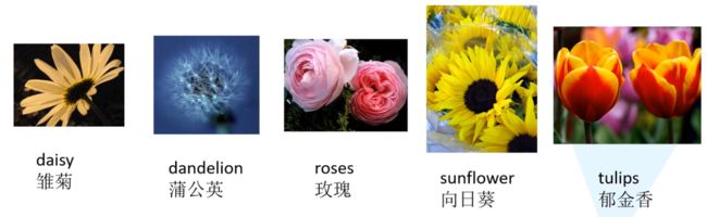
包含 5 中类型的花,每种类型有600~900张图像不等。
训练集与测试集划分
参考:https://github.com/WZMIAOMIAO/deep-learning-for-image-processing/blob/master/data_set/README.md
由于此数据集不像 CIFAR10 那样下载时就划分好了训练集和测试集,因此需要自己划分。
shift + 右键 打开 PowerShell ,执行 “split_data.py” 分类脚本自动将数据集划分成 训练集train 和 验证集val。

 完整的目录结构如下:
|-- flower_data
	|-- flower_photos
		|-- daisy
		|-- dandelion
		|-- roses
		|-- sunflowers
		|-- tulips
		|-- LICENSE.txt
	|-- train
		|-- daisy
		|-- dandelion
		|-- roses
		|-- sunflowers
		|-- tulips
	|-- val
		|-- daisy
		|-- dandelion
		|-- roses
		|-- sunflowers
		|-- tulips
	|-- flower_photos.tgz
|-- flower_link.txt
|-- README.md
|-- split_data.py
split_data.py的代码如下,在用到自己的数据集时,可以简单修改代码中的文件夹名称进行数据集的划分。
import os
from shutil import copy
import random

def mkfile(file):
    if not os.path.exists(file):
        os.makedirs(file)

# 获取 flower_photos 文件夹下除 .txt 文件以外所有文件夹名(即5种花的类名)
file_path = 'flower_data/flower_photos'
flower_class = [cla for cla in os.listdir(file_path) if ".txt" not in cla]

# 创建 训练集train 文件夹,并由5种类名在其目录下创建5个子目录
mkfile('flower_data/train')
for cla in flower_class:
    mkfile('flower_data/train/'+cla)

# 创建 验证集val 文件夹,并由5种类名在其目录下创建5个子目录
mkfile('flower_data/val')
for cla in flower_class:
    mkfile('flower_data/val/'+cla)

# 划分比例,训练集 : 验证集 = 9 : 1
split_rate = 0.1

# 遍历5种花的全部图像并按比例分成训练集和验证集
for cla in flower_class:
    cla_path = file_path + '/' + cla + '/'  # 某一类别花的子目录
    images = os.listdir(cla_path)		    # iamges 列表存储了该目录下所有图像的名称
    num = len(images)
    eval_index = random.sample(images, k=int(num*split_rate)) # 从images列表中随机抽取 k 个图像名称
    for index, image in enumerate(images):
    	# eval_index 中保存验证集val的图像名称
        if image in eval_index:
            image_path = cla_path + image
            new_path = 'flower_data/val/' + cla
            copy(image_path, new_path)  # 将选中的图像复制到新路径

        # 其余的图像保存在训练集train中
        else:
            image_path = cla_path + image
            new_path = 'flower_data/train/' + cla
            copy(image_path, new_path)
        print("\r[{}] processing [{}/{}]".format(cla, index+1, num), end="")  # processing bar
    print()

print("processing done!")
AlexNet详解
AlexNet 是2012年 ISLVRC ( ImageNet Large Scale Visual Recognition Challenge)竞赛的冠军网络,分类准确率由传统的70%+提升到80%+。它是由Hinton和他的学生Alex Krizhevsky设计的。 也是在那年之后,深度学习开始迅速发展。

使用Dropout的方式在网络正向传播过程中随机失活一部分神经元,以减少过拟合

Conv1

注意:原作者实验时用了两块GPU并行计算,上下两组图的结构是一样的。
- 输入:input_size = [224, 224, 3]
- 卷积层:
- kernels = 48 * 2 = 96 组卷积核
- kernel_size = 11
- padding = [1, 2] (左上围加半圈0,右下围加2倍的半圈0)
- stride = 4
- 输出:output_size = [55, 55, 96]
经 Conv1 卷积后的输出层尺寸为:
O u t p u t = ( W − F + 2 P ) S + 1 = [ 224 − 11 + ( 1 + 2 ) ] 4 + 1 = 55 Output = \frac{(W − F + 2P )}{S} + 1 = \frac{[224 − 11 + (1+2)]}{4} + 1 = 55 Output=S(W−F+2P)+1=4[224−11+(1+2)]+1=55
- 输入图片大小 W×W(一般情况下Width=Height)
- Filter大小F×F
- 步长 S
- padding的像素数 P
Maxpool1

- 输入:input_size = [55, 55, 96]
- 池化层:(只改变尺寸,不改变深度channel)
- kernel_size = 3
- padding = 0
- stride = 2
- 输出:output_size = [27, 27, 96]
经 Maxpool1 后的输出层尺寸为:
O u t p u t = ( W − F + 2 P ) S + 1 = ( 55 − 3 ) 2 + 1 = 27 Output = \frac{(W − F + 2P )}{S} + 1 = \frac{(55-3)}{2} + 1 = 27 Output=S(W−F+2P)+1=2(55−3)+1=27
Conv2

- 输入:input_size = [27, 27, 96]
- 卷积层:
- kernels = 128 * 2 = 256 组卷积核
- kernel_size = 5
- padding = [2, 2]
- stride = 1
- 输出:output_size = [27, 27, 256]
经 Conv2 卷积后的输出层尺寸为:
O u t p u t = ( W − F + 2 P ) S + 1 = [ 27 − 5 + ( 2 + 2 ) ] 1 + 1 = 27 Output = \frac{(W − F + 2P )}{S} + 1 = \frac{[27− 5 + (2+2)]}{1} + 1 = 27 Output=S(W−F+2P)+1=1[27−5+(2+2)]+1=27
Maxpool2

- 输入:input_size = [27, 27, 256]
- 池化层:(只改变尺寸,不改变深度channel)
- kernel_size = 3
- padding = 0
- stride = 2
- 输出:output_size = [13, 13, 256]
经 Maxpool2 后的输出层尺寸为:
O u t p u t = ( W − F + 2 P ) S + 1 = ( 27 − 3 ) 2 + 1 = 13 Output = \frac{(W − F + 2P )}{S} + 1 = \frac{(27-3)}{2} + 1 = 13 Output=S(W−F+2P)+1=2(27−3)+1=13
Conv3

- 输入:input_size = [13, 13, 256]
- 卷积层:
- kernels = 192* 2 = 384 组卷积核
- kernel_size = 3
- padding = [1, 1]
- stride = 1
- 输出:output_size = [13, 13, 384]
经 Conv3 卷积后的输出层尺寸为:
O u t p u t = ( W − F + 2 P ) S + 1 = [ 13 − 3 + ( 1 + 1 ) ] 1 + 1 = 13 Output = \frac{(W − F + 2P )}{S} + 1 = \frac{[13− 3 + (1+1)]}{1} + 1 = 13 Output=S(W−F+2P)+1=1[13−3+(1+1)]+1=13
Conv4

- 输入:input_size = [13, 13, 384]
- 卷积层:
- kernels = 192* 2 = 384 组卷积核
- kernel_size = 3
- padding = [1, 1]
- stride = 1
- 输出:output_size = [13, 13, 384]
经 Conv4 卷积后的输出层尺寸为:
O u t p u t = ( W − F + 2 P ) S + 1 = [ 13 − 3 + ( 1 + 1 ) ] 1 + 1 = 13 Output = \frac{(W − F + 2P )}{S} + 1 = \frac{[13− 3 + (1+1)]}{1} + 1 = 13 Output=S(W−F+2P)+1=1[13−3+(1+1)]+1=13
Conv5

- 输入:input_size = [13, 13, 384]
- 卷积层:
- kernels = 128* 2 = 256 组卷积核
- kernel_size = 3
- padding = [1, 1]
- stride = 1
- 输出:output_size = [13, 13, 256]
经 Conv5 卷积后的输出层尺寸为:
O u t p u t = ( W − F + 2 P ) S + 1 = [ 13 − 3 + ( 1 + 1 ) ] 1 + 1 = 13 Output = \frac{(W − F + 2P )}{S} + 1 = \frac{[13− 3 + (1+1)]}{1} + 1 = 13 Output=S(W−F+2P)+1=1[13−3+(1+1)]+1=13
Maxpool3

- 输入:input_size = [13, 13, 256]
- 池化层:(只改变尺寸,不改变深度channel)
- kernel_size = 3
- padding = 0
- stride = 2
- 输出:output_size = [6, 6, 256]
经 Maxpool3 后的输出层尺寸为:
O u t p u t = ( W − F + 2 P ) S + 1 = ( 13 − 3 ) 2 + 1 = 6 Output = \frac{(W − F + 2P )}{S} + 1 = \frac{(13-3)}{2} + 1 = 6 Output=S(W−F+2P)+1=2(13−3)+1=6
FC1、FC2、FC3
Maxpool3 → (6*6*256) → FC1 → 2048 → FC2 → 2048 → FC3 → 1000
最终的1000可以根据数据集的类别数进行修改。
总结

分析可以发现,除 Conv1 外,AlexNet 的其余卷积层都是在改变特征矩阵的深度,而池化层则只改变(减小)其尺寸。
1. model.py
代码中需要注意的是:
- pytorch 中 Tensor 参数的顺序为
(batch, channel, height, width),下面代码中没有写batch - 卷积的参数为
Conv2d(in_channels, out_channels, kernel_size, stride, padding, ...),一般关心这5个参数即可 - 卷积池化层提取图像特征,全连接层进行图像分类,代码中写成两个模块,方便调用
- 为了加快训练,代码只使用了一半的网络参数,相当于只用了原论文中网络结构的下半部分(正好原论文中用的双GPU,我的电脑只有一块GPU)(后来我又用完整网络跑了遍,发现一半参数跟完整参数的训练结果acc相差无几)
import torch.nn as nn
import torch

class AlexNet(nn.Module):
    def __init__(self, num_classes=1000, init_weights=False):
        super(AlexNet, self).__init__()
        # 用nn.Sequential()将网络打包成一个模块,精简代码
        self.features = nn.Sequential(   # 卷积层提取图像特征
            nn.Conv2d(3, 48, kernel_size=11, stride=4, padding=2),  # input[3, 224, 224]  output[48, 55, 55]
            nn.ReLU(inplace=True), 									# 直接修改覆盖原值,节省运算内存
            nn.MaxPool2d(kernel_size=3, stride=2),                  # output[48, 27, 27]
            nn.Conv2d(48, 128, kernel_size=5, padding=2),           # output[128, 27, 27]
            nn.ReLU(inplace=True),
            nn.MaxPool2d(kernel_size=3, stride=2),                  # output[128, 13, 13]
            nn.Conv2d(128, 192, kernel_size=3, padding=1),          # output[192, 13, 13]
            nn.ReLU(inplace=True),
            nn.Conv2d(192, 192, kernel_size=3, padding=1),          # output[192, 13, 13]
            nn.ReLU(inplace=True),
            nn.Conv2d(192, 128, kernel_size=3, padding=1),          # output[128, 13, 13]
            nn.ReLU(inplace=True),
            nn.MaxPool2d(kernel_size=3, stride=2),                  # output[128, 6, 6]
        )
        self.classifier = nn.Sequential(   # 全连接层对图像分类
            nn.Dropout(p=0.5),			   # Dropout 随机失活神经元,默认比例为0.5
            nn.Linear(128 * 6 * 6, 2048),
            nn.ReLU(inplace=True),
            nn.Dropout(p=0.5),
            nn.Linear(2048, 2048),
            nn.ReLU(inplace=True),
            nn.Linear(2048, num_classes),
        )
        if init_weights:
            self._initialize_weights()

	# 前向传播过程
    def forward(self, x):
        x = self.features(x)
        x = torch.flatten(x, start_dim=1)	# 展平后再传入全连接层
        x = self.classifier(x)
        return x

	# 网络权重初始化,实际上 pytorch 在构建网络时会自动初始化权重
    def _initialize_weights(self):
        for m in self.modules():
            if isinstance(m, nn.Conv2d):                            # 若是卷积层
                nn.init.kaiming_normal_(m.weight, mode='fan_out',   # 用(何)kaiming_normal_法初始化权重
                                        nonlinearity='relu')
                if m.bias is not None:
                    nn.init.constant_(m.bias, 0)                    # 初始化偏重为0
            elif isinstance(m, nn.Linear):            # 若是全连接层
                nn.init.normal_(m.weight, 0, 0.01)    # 正态分布初始化
                nn.init.constant_(m.bias, 0)          # 初始化偏重为0
2. train.py
# 导入包
import torch
import torch.nn as nn
from torchvision import transforms, datasets, utils
import matplotlib.pyplot as plt
import numpy as np
import torch.optim as optim
from model import AlexNet
import os
import json
import time

# 使用GPU训练
device = torch.device("cuda" if torch.cuda.is_available() else "cpu")
print(device)
2.1 数据预处理
需要注意的是,对训练集的预处理,多了随机裁剪和水平翻转这两个步骤。可以起到扩充数据集的作用,增强模型泛化能力。
参考:Pytorch中transforms.RandomResizedCrop()等图像操作
data_transform = {
    "train": transforms.Compose([transforms.RandomResizedCrop(224),       # 随机裁剪,再缩放成 224×224
                                 transforms.RandomHorizontalFlip(p=0.5),  # 水平方向随机翻转,概率为 0.5, 即一半的概率翻转, 一半的概率不翻转
                                 transforms.ToTensor(),
                                 transforms.Normalize((0.5, 0.5, 0.5), (0.5, 0.5, 0.5))]),

    "val": transforms.Compose([transforms.Resize((224, 224)),  # cannot 224, must (224, 224)
                               transforms.ToTensor(),
                               transforms.Normalize((0.5, 0.5, 0.5), (0.5, 0.5, 0.5))])}
2.2 导入、加载 训练集
还记得上篇用到的 CIFAR10 是怎么导入和加载数据集的吗?
上篇LeNet网络搭建中是使用的torchvision.datasets.CIFAR10和torch.utils.data.DataLoader()来导入和加载数据集。
# 导入训练集
train_set = torchvision.datasets.CIFAR10(root='./data', 	 # 数据集存放目录
										 train=True,		 # 表示是数据集中的训练集
                                        download=True,  	 # 第一次运行时为True,下载数据集,下载完成后改为False
                                        transform=transform) # 预处理过程
# 加载训练集
train_loader = torch.utils.data.DataLoader(train_set, 	  # 导入的训练集
										   batch_size=50, # 每批训练的样本数
                                          shuffle=False,  # 是否打乱训练集
                                          num_workers=0)  # num_workers在windows下设置为0
但是这次的 花分类数据集 并不在 pytorch 的 torchvision.datasets. 中,因此需要用到datasets.ImageFolder()来导入。
ImageFolder()返回的对象是一个包含数据集所有图像及对应标签构成的二维元组容器,支持索引和迭代,可作为torch.utils.data.DataLoader的输入。具体可参考:pytorch ImageFolder和Dataloader加载自制图像数据集
# 获取图像数据集的路径
data_root = os.path.abspath(os.path.join(os.getcwd(), "../.."))  		# get data root path 返回上上层目录
image_path = data_root + "/data_set/flower_data/"  				 		# flower data_set path

# 导入训练集并进行预处理
train_dataset = datasets.ImageFolder(root=image_path + "/train",
                                     transform=data_transform["train"])
train_num = len(train_dataset)

# 按batch_size分批次加载训练集
train_loader = torch.utils.data.DataLoader(train_dataset,	# 导入的训练集
                                           batch_size=32, 	# 每批训练的样本数
                                           shuffle=True,	# 是否打乱训练集
                                           num_workers=0)	# 使用线程数,在windows下设置为0
2.3 导入、加载 验证集
# 导入验证集并进行预处理
validate_dataset = datasets.ImageFolder(root=image_path + "/val",
                                        transform=data_transform["val"])
val_num = len(validate_dataset)

# 加载验证集
validate_loader = torch.utils.data.DataLoader(validate_dataset,	# 导入的验证集
                                              batch_size=32,
                                              shuffle=True,
                                              num_workers=0)
2.4 存储 索引:标签 的字典
为了方便在 predict 时读取信息,将 索引:标签 存入到一个 json 文件中
# 字典,类别:索引 {'daisy':0, 'dandelion':1, 'roses':2, 'sunflower':3, 'tulips':4}
flower_list = train_dataset.class_to_idx
# 将 flower_list 中的 key 和 val 调换位置
cla_dict = dict((val, key) for key, val in flower_list.items())

# 将 cla_dict 写入 json 文件中
json_str = json.dumps(cla_dict, indent=4)
with open('class_indices.json', 'w') as json_file:
    json_file.write(json_str)
class_indices.json 文件内容如下:
{
    "0": "daisy",
    "1": "dandelion",
    "2": "roses",
    "3": "sunflowers",
    "4": "tulips"
}
2.5 训练过程
训练过程中需要注意:
net.train():训练过程中开启 Dropoutnet.eval(): 验证过程关闭 Dropout
net = AlexNet(num_classes=5, init_weights=True)  	  # 实例化网络(输出类型为5,初始化权重)
net.to(device)									 	  # 分配网络到指定的设备(GPU/CPU)训练
loss_function = nn.CrossEntropyLoss()			 	  # 交叉熵损失
optimizer = optim.Adam(net.parameters(), lr=0.0002)	  # 优化器(训练参数,学习率)

save_path = './AlexNet.pth'
best_acc = 0.0

for epoch in range(10):
    ########################################## train ###############################################
    net.train()     					# 训练过程中开启 Dropout
    running_loss = 0.0					# 每个 epoch 都会对 running_loss  清零
    time_start = time.perf_counter()	# 对训练一个 epoch 计时

    for step, data in enumerate(train_loader, start=0):  # 遍历训练集,step从0开始计算
        images, labels = data   # 获取训练集的图像和标签
        optimizer.zero_grad()	# 清除历史梯度

        outputs = net(images.to(device))				 # 正向传播
        loss = loss_function(outputs, labels.to(device)) # 计算损失
        loss.backward()								     # 反向传播
        optimizer.step()								 # 优化器更新参数
        running_loss += loss.item()

        # 打印训练进度(使训练过程可视化)
        rate = (step + 1) / len(train_loader)           # 当前进度 = 当前step / 训练一轮epoch所需总step
        a = "*" * int(rate * 50)
        b = "." * int((1 - rate) * 50)
        print("\rtrain loss: {:^3.0f}%[{}->{}]{:.3f}".format(int(rate * 100), a, b, loss), end="")
    print()
    print('%f s' % (time.perf_counter()-time_start))

    ########################################### validate ###########################################
    net.eval()    # 验证过程中关闭 Dropout
    acc = 0.0
    with torch.no_grad():
        for val_data in validate_loader:
            val_images, val_labels = val_data
            outputs = net(val_images.to(device))
            predict_y = torch.max(outputs, dim=1)[1]  # 以output中值最大位置对应的索引(标签)作为预测输出
            acc += (predict_y == val_labels.to(device)).sum().item()
        val_accurate = acc / val_num

        # 保存准确率最高的那次网络参数
        if val_accurate > best_acc:
            best_acc = val_accurate
            torch.save(net.state_dict(), save_path)

        print('[epoch %d] train_loss: %.3f  test_accuracy: %.3f \n' %
              (epoch + 1, running_loss / step, val_accurate))

print('Finished Training')
训练打印信息如下:
cuda
train loss: 100%[**************************************************->]1.566
27.450399 s
[epoch 1] train_loss: 1.413  test_accuracy: 0.404

train loss: 100%[**************************************************->]1.412
27.897467399999996 s
[epoch 2] train_loss: 1.211  test_accuracy: 0.503

train loss: 100%[**************************************************->]1.412
28.665594 s
[epoch 3] train_loss: 1.138  test_accuracy: 0.544

train loss: 100%[**************************************************->]0.924
28.6858524 s
[epoch 4] train_loss: 1.075  test_accuracy: 0.621

train loss: 100%[**************************************************->]1.200
28.020624199999986 s
[epoch 5] train_loss: 1.009  test_accuracy: 0.621

train loss: 100%[**************************************************->]0.985
27.973145999999986 s
[epoch 6] train_loss: 0.948  test_accuracy: 0.607

train loss: 100%[**************************************************->]0.583
28.290610200000003 s
[epoch 7] train_loss: 0.914  test_accuracy: 0.670

train loss: 100%[**************************************************->]0.930
28.51416950000001 s
[epoch 8] train_loss: 0.912  test_accuracy: 0.621

train loss: 100%[**************************************************->]1.210
28.98158360000002 s
[epoch 9] train_loss: 0.840  test_accuracy: 0.668

train loss: 100%[**************************************************->]0.961
28.330670499999997 sp
[epoch 10] train_loss: 0.833  test_accuracy: 0.684

Finished Training
3. predict.py
import torch
from model import AlexNet
from PIL import Image
from torchvision import transforms
import matplotlib.pyplot as plt
import json

# 预处理
data_transform = transforms.Compose(
    [transforms.Resize((224, 224)),
     transforms.ToTensor(),
     transforms.Normalize((0.5, 0.5, 0.5), (0.5, 0.5, 0.5))])

# load image
img = Image.open("蒲公英.jpg")
plt.imshow(img)
# [N, C, H, W]
img = data_transform(img)
# expand batch dimension
img = torch.unsqueeze(img, dim=0)

# read class_indict
try:
    json_file = open('./class_indices.json', 'r')
    class_indict = json.load(json_file)
except Exception as e:
    print(e)
    exit(-1)

# create model
model = AlexNet(num_classes=5)
# load model weights
model_weight_path = "./AlexNet.pth"
model.load_state_dict(torch.load(model_weight_path))

# 关闭 Dropout
model.eval()
with torch.no_grad():
    # predict class
    output = torch.squeeze(model(img))     # 将输出压缩,即压缩掉 batch 这个维度
    predict = torch.softmax(output, dim=0)
    predict_cla = torch.argmax(predict).numpy()
print(class_indict[str(predict_cla)], predict[predict_cla].item())
plt.show()
打印出预测的标签以及概率值:
dandelion 0.7221569418907166