kaggle-2美国人口普查年收入50K分类

本文主要是使用xgboost， RandomForestClassifier算法实现美国1994年人口普查数据，居民年收入是否超过50K的分类问题。

主要内容如下:

1 数据预处理

• 数据信息查看，添加对应的列标签

• 缺失值处理，以及属性值替换

• Ordinal Encoding to Categoricals（string 特征转化为整数编码）

2 模型训练以及验证

• xgboost算法分类以及GridSearchCV 参数寻优

• xgboost early stopping CV

• 测试集准确率验证

• RandomForestClassifier模型分类以及验证

---

1 数据预处理

1.1 数据描述

数据集说明以及下载地址：
https://archive.ics.uci.edu/ml/datasets/Adult
https://archive.ics.uci.edu/ml/machine-learning-databases/adult/

该数据从美国1994年人口普查数据库抽取而来，可以用来预测居民收入是否超过50K /year。该数据集类变量为年收入是否超过50k ，属性变量包含年龄，工种，学历，职业，人种等重要信息，值得一提的是，14个属性变量中有7个类别型变量.
数据集各属性是:其中序号0~13是属性， 14是类别

序号	字段名	含义	类型
0	age	年龄	Double
1	workclass	工作类型*	string
2	fnlwgt	序号	string
3	education	教育程度*	string
4	education_num	受教育时间	double
5	maritial_status	婚姻状况*	string
6	occupation	职业*	string
7	relationship	关系*	string
8	race	种族*	string
9	sex	性别*	string
10	capital_gain	资本收益	string
11	capital_loss	资本损失	string
12	hours_per_week	每周工作小时数	double
13	native_country	原籍*	string
14(label)	income	收入	string

---

1.2 load data

def get_data():
    train_path = "./dataset/adult.data"
    test_path = './dataset/adult.test'

    train_set = pd.read_csv(train_path, header=None)
    print train_set.head()

数据前五行输出如下:

   0                  1       2           3   4                   5   
0  39          State-gov   77516    Bachelors  13        Never-married   
1  50    Self-emp-not-inc   83311    Bachelors  13     Married-civ-spouse   
2  38            Private  215646     HS-grad   9             Divorced   
3  53            Private  234721        11th   7     Married-civ-spouse   
4  28            Private  338409    Bachelors  13     Married-civ-spouse   

........省略
               13      14  
0   United-States   <=50K  
1   United-States   <=50K  
2   United-States   <=50K  
3   United-States   <=50K  
4         Cuba    <=50K  

测试数据集这里不给出输出，太多了，数据集问题:

1. 数据没有column name

2. 测试集中有缺失值，

下面给数据集添加列标签

col_labels = ['age', 'workclass', 'fnlwgt', 'education', 'education_num', 'marital_status',
              'occupation', 'relationship', 'race', 'sex', 'capital_gain', 'capital_loss',
              'hours_per_week', 'native_country', 'wage_class']

train_set.columns = col_labels
test_set.columns = col_labels

print train_set.info()
print test_set.info()

下面仅给出测试集的信息(中间部分省略)

Data columns (total 15 columns):
age               16281 non-null int64
workclass         16281 non-null object
.................
wage_class        16281 non-null object
dtypes: int64(6), object(9)
memory usage: 1.9+ MB

1.3 缺失值处理

训练集以及测试集中的缺失值都是用 ? 替换的，首先将其移除:

print train_set.replace(' ?', np.nan).dropna().shape
# (30162, 15)
print test_set.replace(' ?', np.nan).dropna().shape
# (15060, 15)

# 删除含有?（缺失行）
train_set = train_set.replace(' ?', np.nan).dropna()

test_set = test_set.replace(' ?', np.nan).dropna()

---

1.4 值替换

替换测试集中的wage_class值使得其与train_set一致

test_set['wage_class'] = test_set.wage_class.replace({' <=50K.': ' <=50K', ' >50K.': ' >50K'})
print test_set.wage_class.unique()
# [' <=50K' ' >50K']
print train_set.wage_class.unique()
# [' <=50K' ' >50K']

print test_set.wage_class.unique()
# [' <=50K' ' >50K']
print train_set.wage_class.unique()
# [' <=50K' ' >50K']

---

1.5 查看列属性和类别的关系

我们可以查看下，教育程度和类别(年收入>=50Kde 关系，一般来说学历越高，年收入高的概率越大)

print train_set.education.unique()

print pd.crosstab(train_set['wage_class'], train_set['education'], rownames=['wage_class'])

输出如下, 教育程度有如下几种:

[' Bachelors' ' HS-grad' ' 11th' ' Masters' ' 9th' ' Some-college'
 ' Assoc-acdm' ' 7th-8th' ' Doctorate' ' Assoc-voc' ' Prof-school'
 ' 5th-6th' ' 10th' ' Preschool' ' 12th' ' 1st-4th']

教育程度和类别关系输出如下:

education    10th   11th   12th   1st-4th   5th-6th   7th-8th   9th  \
wage_class                                                            
 <=50K        761    989    348       145       276       522   430   
 >50K          59     59     29         6        12        35    25   

......................................
education    Masters   Preschool   Prof-school   Some-college  
wage_class                                                     
 <=50K           709          45           136           5342  
 >50K            918           0           406           1336  

我们可以看到Masters(研究生)的>=50K的比例较高，而Preschool没有上个学的基本没有>=50K的。

---

1.6 Ordinal Encoding to Categoricals

字符串类型转化为数值类型,为了保证测试集和训练集的encoding类型一致，我们首先将两个表join，编码完成之后，在分开到原始的表中:

combined_set = pd.concat([train_set, test_set], axis=0)

合并完成将表中的object数据转化为int类型：

for feature in combined_set.columns:
    if combined_set[feature].dtype == 'object':
        combined_set[feature] = pd.Categorical(combined_set[feature]).codes

将数据转到原有的训练集以及测试集中:

train_set = combined_set[:train_set.shape[0]]
test_set = combined_set[train_set.shape[0]:]

我们可以看下，education以及wage_class的编码:

print train_set.education.unique()
print train_set.wage_class.unique()

输出如下：

[ 9 11  1 12  6 15  7  5 10  8 14  4  0 13  2  3]
[0 1]

---

2 模型训练以及验证

2.1 xgboost算法分类以及GridSearchCV 参数寻优

生成训练集以及测试集：

y_train = train_set.pop('wage_class')
y_set = test_set.pop('wage_class')

return train_set, y_train, test_set, y_set

xgboost结合GridSearchCV参数寻优：

def train_validate(X_train, Y_train, X_test, Y_test):
    cv_params = {'max_depth': [3, 5, 7], 'min_child_weight': [1, 3, 5]}
    ind_params = {'learning_rate': 0.1, 'n_estimators': 1000, 'seed': 0,
                  'subsample': 0.8, 'colsample_bytree': 0.8,
                  'objective': 'binary:logistic'}

    import os
    mingw_path = 'C:/Program Files/mingw-w64/x86_64-6.2.0-posix-seh-rt_v5-rev1/mingw64/bin'
    os.environ['PATH'] = mingw_path + ';' + os.environ['PATH']
    print os.environ['PATH'].count(mingw_path)
    from xgboost import XGBClassifier

    optimized_GBM = GridSearchCV(XGBClassifier(**ind_params),
                                 cv_params,
                                 scoring='accuracy', cv=5, n_jobs=-1)

使用5-fold cross-validation，查看最佳参数:

optimized_GBM.fit(X_train, Y_train)

参数以及结果输出:

print optimized_GBM.best_params_

for params, mean_score, scores in optimized_GBM.grid_scores_:
    print("%0.3f (+/-%0.03f) for %r"
          % (mean_score, scores.std() * 2, params))

输出如下:

{'max_depth': 3, 'min_child_weight': 5}

0.867 (+/-0.005) for {'max_depth': 3, 'min_child_weight': 1}
0.867 (+/-0.007) for {'max_depth': 3, 'min_child_weight': 3}
0.867 (+/-0.006) for {'max_depth': 3, 'min_child_weight': 5}
0.862 (+/-0.006) for {'max_depth': 5, 'min_child_weight': 1}
0.860 (+/-0.005) for {'max_depth': 5, 'min_child_weight': 3}
0.862 (+/-0.005) for {'max_depth': 5, 'min_child_weight': 5}
0.856 (+/-0.007) for {'max_depth': 7, 'min_child_weight': 1}
0.855 (+/-0.006) for {'max_depth': 7, 'min_child_weight': 3}
0.857 (+/-0.006) for {'max_depth': 7, 'min_child_weight': 5}

预测测试数据:

Y_pred = optimized_GBM.predict(X_test)
print classification_report(Y_test, Y_pred)

输出如下:

               precision  recall  f1-score   support
          0       0.90      0.94      0.91     11360
          1       0.77      0.66      0.71      3700
avg / total       0.86      0.87      0.87     15060

接下来，我们在最优参数{‘max_depth’: 3, ‘min_child_weight’: 5}，条件下调整learning_rate， 以及subsample：

cv_params = {'learning_rate': [0.1, 0.05, 0.01], 'subsample': [0.7, 0.8, 0.9]}
ind_params = {'max_depth': 3, 'n_estimators': 1000, 'seed': 0,'min_child_weight': 1, 'colsample_bytree': 0.8, 'objective': 'binary:logistic'}

输出结果如下:

{'subsample': 0.8, 'learning_rate': 0.05}

0.866 (+/-0.005) for {'subsample': 0.7, 'learning_rate': 0.1}
..................省略
0.868 (+/-0.005) for {'subsample': 0.7, 'learning_rate': 0.05}
0.869 (+/-0.006) for {'subsample': 0.8, 'learning_rate': 0.05}
..................省略
0.860 (+/-0.006) for {'subsample': 0.9, 'learning_rate': 0.01}

             precision    recall  f1-score   support
          0       0.89      0.94      0.91     11360
          1       0.77      0.66      0.71      3700
avg / total       0.86      0.87      0.86     15060

可以看到在{‘max_depth’: 3, ‘min_child_weight’: 5}条件下, {‘subsample’: 0.8, ‘learning_rate’: 0.05}为最佳参数(当然感兴趣的话，你也可以，在做更多的参数组合)。

---

2.2 xgboost early stopping CV防止过拟合

接下来我们使用上面的参数，并使用xgboost原生的参数

# 训练集使用xgboost原生的形式(性能的提升)
xgdmat = xgb.DMatrix(train_set, y_train)

our_params = {'eta': 0.05, 'seed':0, 'subsample': 0.8, 'colsample_bytree': 0.8,
              'objective': 'binary:logistic', 'max_depth': 3, 'min_child_weight': 1}

cv_xgb = xgb.cv(params=our_params, dtrain=xgdmat, num_boost_round=3000, nfold=5,
                metrics=['error'],
                early_stopping_rounds=100)  # Look for early stopping that minimizes error)

# 查看输出结果，后五行：
print cv_xgb.tail(5)

输出如下:

       test-error-mean      test-error-std    train-error-mean     train-error-std
598         0.131225        0.004856          0.121859         0.001241
599         0.131291        0.004765          0.121842         0.001190
600         0.131125        0.004791          0.121875         0.001181
601         0.131125        0.004787          0.121875         0.001222
602         0.131092        0.004846          0.121834         0.001246

final_gb = xgb.train(our_params, xgdmat, num_boost_round=602)
xgb.plot_importance(final_gb)
plt.show()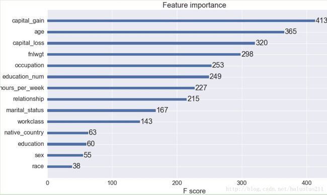

可见capital_gain的影响因数最大（一般有资本收益的，当然往往收入会比较高），这点比较符合常识。

2.3 测试集准确率验证

testdmat = xgb.DMatrix(test_set)
y_pred = final_gb.predict(testdmat)
print y_pred

y_pred[y_pred > 0.5] = 1
y_pred[y_pred <= 0.5] = 0

print classification_report(y_pred, y_set)

输出的是概率

[ 0.00376732  0.22359528  0.29395726 ...,  0.81296259  0.17736618
  0.79582822]

准确率如下:

              precision     recall  f1-score   support
        0.0       0.94      0.89      0.91     12059
        1.0       0.64      0.78      0.70      3001
avg / total       0.88      0.87      0.87     15060

---

2.4 RandomForestClassifier模型分类以及验证

代码如下，没有做任何的参数调优

def rfc_fit_test(X_train, X_test, Y_train, Y_test):
    from sklearn.ensemble import RandomForestClassifier
    rf = RandomForestClassifier(n_jobs=4)
    rf.fit(X_train, Y_train)
    Y_pred = rf.predict(X_test)
    print classification_report(Y_test, Y_pred)

输出如下:

               precision    recall  f1-score   support
          0       0.87      0.93      0.90     11360
          1       0.73      0.59      0.65      3700
avg / total       0.84      0.85      0.84     15060

识别率为84%

参考:

思路以及代码大部分参考下面这篇blog:
https://jessesw.com/XG-Boost/

xgboost官方文档
https://xgboost.readthedocs.io/en/latest/

下面这个网站专门可以生成markdown的table(支持word的table复制，粘贴)
https://www.tablesgenerator.com/markdown_tables