特征选择：Boston house prices 数据集分析(R 语言)

How the choose the features?

怎样选择特征?

• construct a multivariate linear model using all the provided features and choose those with 0.001 significance level(or 0.01, 0.05 significance level)
• 使用所有的特征建立多元线性回归模型并且选择那些具有高显著性的特征
• plotting the dependent variable vs each of the chosen features and explore the potential correlation (like logarithm, polynomial)
• 绘制待预测变量与每一个选择的特征的图像并且探索图像中潜在的关系（如指数关系、n次多项式关系）
• construct the covariance matrix and make an interaction of those with high correlation
• 构建相关系数矩阵并且将相关性高的特征乘起来

General Implementation with R

R 语言实现

# import some necessary packages
library(haven) # used to load our data
library(texreg) # used to display fit info
library(dplyr) # used to manipulate data
library(tidyr) # used for the drop_na function
library(ggplot2) # in case we want to make ggplots
library(caTools)
library(MASS)
library(corrgram)

# import Boston dataset
boston_df <- Boston

# change the name of the columns
names(boston_df) <- c("crime", "zoned_bigger_25000", "non_retail_proportion","chas_river", "nitrogen_density", "average_room_number", "built_before_1940_ratio", "distance_to_centre", "accessbility_to_highway", "tax_rate", "pupil_teacher_ratio", "black_formula","lower_class_ratio", "median_house_price")

# change the category features into factor 
boston_df$chas_river <- factor(boston_df$chas_river, c(1, 0), c("tract bounds river", "not tract bounds river"))

# make a summary of the whole dataset
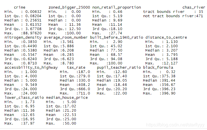
summary(boston_df)

Using all the features to construct a multivariate model

model_all <- lm(median_house_price ~ ., data = train)
summary(model_all)

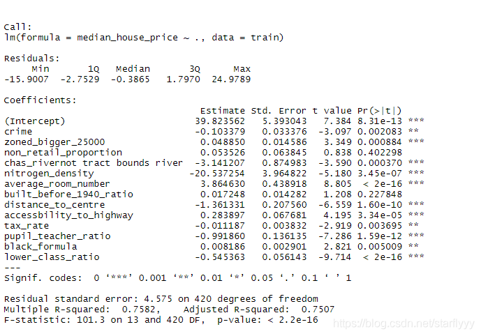
We can find that average_room_number and lower_class_ratio have the biggest significance level so we first explore those two features.

Plotting the dependent variable vs each of the chosen features and explore the potential correlation (like logarithm, polynomial)

# plot the median_house_price vs. average_room_number
plot(train$average_room_number, train$median_house_price)

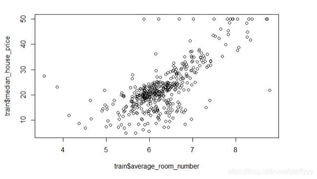
The specific relationship is hard to determine in this figure. So just try logarithm, polynomial.
In my case, I find that the Quaternion polynomial may be the best choice.

model.good.average_room_number <- lm(median_house_price ~ poly(average_room_number, 4), data = train)
screenreg(model.good.average_room_number)

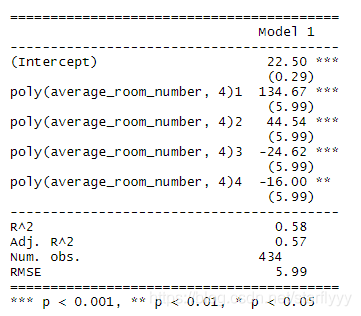
Again, I explore the feature lower_class_ratio.

plot(train$lower_class_ratio, train$median_house_price)

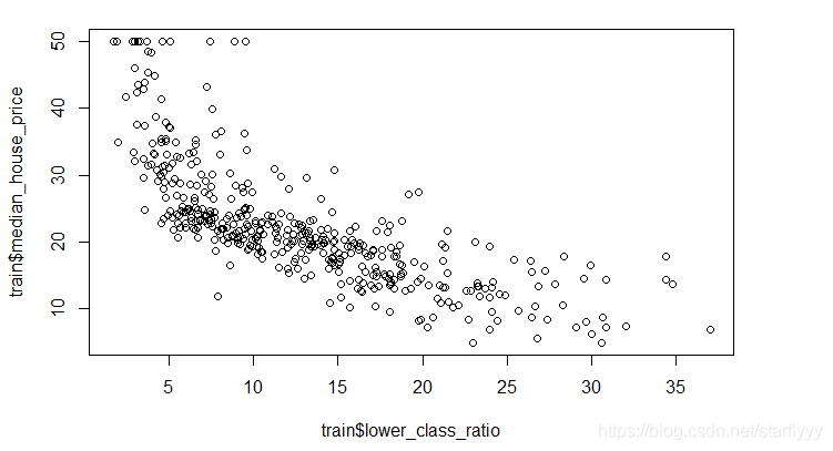
In this case, a logarithm relationship may works(also you can try polynomials)

model.good.lower_class_ratio <- lm(median_house_price ~ log(lower_class_ratio), data = train)
screenreg(model.good.lower_class_ratio)

We can find that the R squared reach to 0.67 which indicates it is an really important feature.
Similarly, we can explore other features.

Construct the covariance matrix and make an interaction of those with high correlation.

library(corrgram)
corrgram(train)
corrgram(train, order = TRUE, lower.panel= panel.shade, upper.panel = panel.pie, main = "correlogram of all predictors")

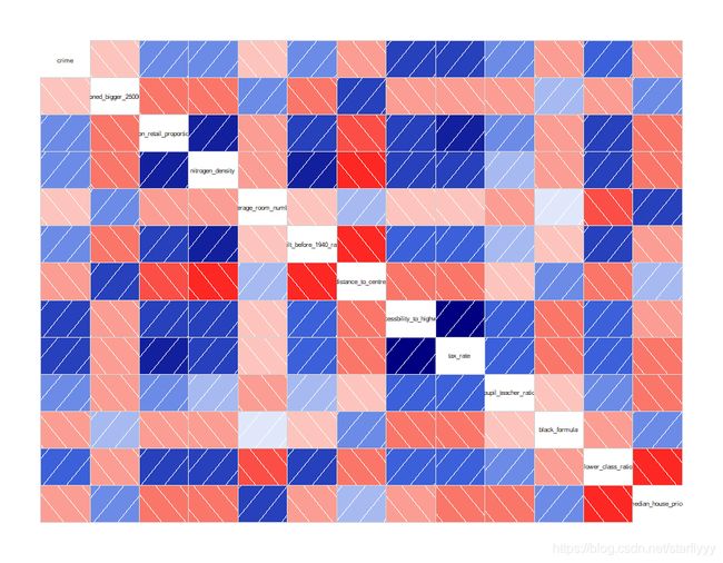
We can find that average_room_number & lower_class_ratio have a high correlation so may put them together.

model.good.lower_interaction_room <- lm(median_house_price ~ log(lower_class_ratio) * poly(average_room_number,4), data = train)
screenreg(model.good.lower_interaction_room)

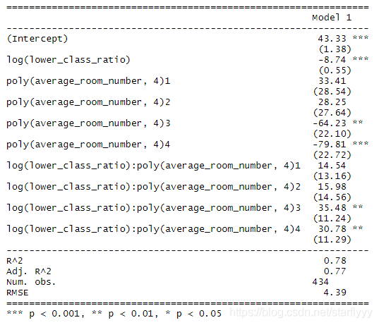
We can find that just using the two features make a good fit.
Then we can finish the remaining features and the result is as follows:

model.maybe.best <- lm(median_house_price ~ pupil_teacher_ratio + nitrogen_density * distance_to_centre + log(lower_class_ratio) * poly(average_room_number,4), data = train)
screenreg(model.maybe.best)

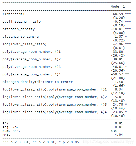
We can find that the final $R^2$ result is 0.81.
Then we use the test dataset to make a prediction.

maybe_prediction <- predict(model.maybe.best, newdata = test)
df <- data.frame(test$median_house_price, maybe_prediction)

#calculate R^2 by myself
rss <- sum((maybe_prediction - test$median_house_price) ^ 2)  ## residual sum of squares
tss <- sum((test$median_house_price - mean(test$median_house_price)) ^ 2)  ## total sum of squares
rsq <- 1 - rss/tss
rsq

the result of the rsq is 0.834.