机器学习之八大算法④——神经网络(二分类BP算法)

二分类BP算法代码及注释

import numpy as np
import matplotlib.pyplot as plt

# 中文、负号
plt.rcParams['font.sans-serif'] = ['SimHei']
plt.rcParams['axes.unicode_minus'] = False

#数据集
x1 = [0.697,0.774,0.634,0.608,0.556,0.403,0.481,0.437,0.666,0.243,0.245,0.343,0.639,0.657,0.360,0.593,0.719]
x2 = [0.460,0.376,0.264,0.318,0.215,0.237,0.149,0.211,0.091,0.267,0.057,0.099,0.161,0.198,0.370,0.042,0.103]
y = [1,1,1,1,1,1,1,1,0,0,0,0,0,0,0,0,0]

#数据提取
x = np.c_[x1,x2]

# 数据预处理
def preProcess(x,y):
    # 特征缩放(标准化)
    x -= np.mean(x,0)
    x /= np.std(x,0,ddof=1)

    # 数据初始化
    x = np.c_[np.ones(len(x)),x]
    y = np.c_[y]
    return x,y
#调用预处理函数
x,y = preProcess(x,y)

# 洗牌
np.random.seed(7)
order = np.random.permutation(len(x))
x = x[order]
y = y[order]

#数据集切分(train/test)
train_x,test_x = np.split(x,[int(0.7*len(x))])
train_y,test_y = np.split(y,[int(0.7*len(x))])

# 正向传播算法
# 激活函数(逻辑函数)
def g(z,deriv=False):
    if deriv:
        return z*(1-z)
    return 1/(1+np.exp(-z))

# 定义模型
def model(x,theta1,theta2,theta3):
    z2 = np.dot(x,theta1)
    a2 = g(z2)
    z3 = np.dot(a2, theta2)
    a3 = g(z3)
    z4 = np.dot(a3, theta3)
    a4 = g(z4)
    return a2,a3,a4

# 代价函数
def costFunc(h,y):
    j = (-1/len(y))*np.sum(y*np.log(h) + (1-y)*np.log(1-h))
    return j

# 向后传播(BP算法)
def BP(a1,a2,a3,a4,theta1,theta2,theta3,alpha,y):
    # 求delta值
    delta4 = a4 - y
    delta3 = np.dot(delta4,theta3.T)*g(a3,True)
    delta2 = np.dot(delta3,theta2.T)*g(a2,True)

    # 求deltaTheta
    deltatheta3 = (1/len(y))*np.dot(a3.T,delta4)
    deltatheta2 = (1/len(y))*np.dot(a2.T,delta3)
    deltatheta1 = (1/len(y))*np.dot(a1.T,delta2)

    # 更新theta
    theta1 -= alpha*deltatheta1
    theta2 -= alpha*deltatheta2
    theta3 -= alpha*deltatheta3
    return theta1,theta2,theta3

# 梯度下降函数
def gradDesc(x,y,alpha=0.7,max_iter=10000,hidden_layer_size=(17,8)):
    m,n = x.shape
    k = y.shape[1]

    # 初始化theta
    theta1 = 2 * np.random.rand(n,hidden_layer_size[0]) - 1
    theta2 = 2 * np.random.rand(hidden_layer_size[0],hidden_layer_size[1]) - 1
    theta3 = 2 * np.random.rand(hidden_layer_size[1],k) - 1

    # 初始化代价
    j_history = np.zeros(max_iter)

    for i in range(max_iter):
        # 求预测值
        a2, a3, a4 = model(x,theta1,theta2,theta3)
        # 记录代价
        j_history[i] = costFunc(a4,y)
        # 反向传播，更新参数
        theta1, theta2, theta3 = BP(x, a2, a3, a4, theta1, theta2, theta3, alpha, y)
    return j_history,theta1, theta2, theta3

#调用梯度下降函数
j_history,theta1, theta2, theta3 = gradDesc(train_x,train_y)

#训练集预测值
train_a2,train_a3,train_h = model(train_x,theta1, theta2, theta3)
#预测结果标签
test_a2,test_a3,test_h = model(test_x,theta1, theta2, theta3)

#定义准确率
def score(h,y):
    count = 0
    for i in range(len(y)):
        if np.where(h[i] >= 0.5,1,0) == y[i]:
            count += 1
    return count/len(y)

print('训练集准确率:',score(train_h,train_y))
print('测试集准确率:',score(test_h,test_y))

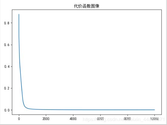
# 画图
plt.title('代价函数图像')
plt.plot(j_history)
plt.show()

---

效果展示

---