车道线检测-从单车道到多车道的车道线检测（一）

车道线检测

····在参加udacity的课程后，对于车道线有了一些直观的认识，后来在实验室学习和外出实习过程中，也接触过不少车道线方面的检测工作，这边将对这些日子里的工作做一个总结。
····这也是我写的第一篇博客（以前都习惯整理在自己电脑里面，但想想还是没有blog绘声绘色）。
····车道线检测，从易到难：单直线车道检测–>单弯道车道检测–>多直线车道检测–>多弯道车道检测（事实上能检测弯道就能够检测直道，相当于曲率半径极大的弯道）
····我更希望用例子去说明，多按图说话。本篇分三个内容：

···· 1.讲解Udacity的CarND-LaneLines-P1-master项目
···· 2.讲解Udacity的CarND-Advanced-Lane-Lines-master项目
···· 3.讲解我在这基础上改进的multi-lane-lines-detection项目

CarND-LaneLines-P1-master

····只能针对直线车道检测，结果稳定，实时性高，但波动大，鲁棒性差，有待改进。

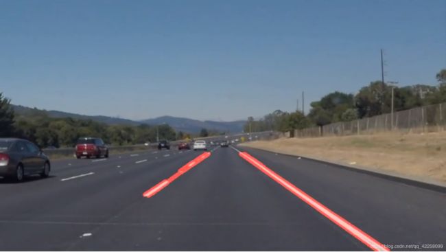
····如图所示，为项目结果图，从单车道检测而言，效果不错而且实时性高，那么具体是怎么做的呢！
····主要思路：对输入图像通过灰度化、高斯滤波、canny边缘检测；再框选出感兴趣区域，对感兴趣区域内的二值化点集进行hough变换，得到目标直线集；对直线集进行分类、合并得到稳定输出结果。

思路讲解

····我们通过一帧图片来说明处理过程。

····如图[image]所示为图像原图，此时为（540x860x3）的数组矩阵，即3层R，G，B通道色彩数据，canny算子变换只关注色值，即（540x860）矩阵中的数值，同一张图片，三通道色值差异不大，通过灰度化，压缩3通道为单通道，减少数据量，使用函数cv2.cvtColor(image, cv2.COLOR_RGB2GRAY)，通常效果较好的是加权平均灰度化，其他具体处理方式见¹，里面通过图例，简单直观说明其原理和方法。；
····对比[gray]、[blur_gray]，明显觉得[blur]更模糊一些，这是由于[blur]进行了高斯滤波，设计一个计算核，大小为3x3或者5x5，类似加权平均的方法，权值满足正态分布，遍历图片，去掉可能存在的椒盐噪声，为hough变换做好准备，这里使用cv2.GaussianBlur(gray, (kernel_size, kernel_size), 0)，实现高斯滤波，kernel_size就是核的大小，一般为基数，有疑惑的童鞋请见转载²，里面通过图例，直观说明常用图像处理滤波器；

····此时，我们转移注意力到图[edges]，[edges]通过边缘检测得到，边缘检测算子常见的有Canny，Roberts，Prewitt，简而言之，通过算子基于差分原理得到一个数值，代表区别度大小，再基于两个阈值对图像进行滤波，去除过多噪点，得到high_threimg和low_threimg，由于high_threshold阈值更大，必然去掉了部分有效特征，再与low_threimg图像进行比对、拼接，得到稳定的图像输出结果，这里使用cv2.Canny(blur_gray, low_threshold, high_threshold)，通过high_threshold和low_threshold对区别度进行限制，实现理想的二值化图[edges]，这里的threshold皆为经验调参值，关于Canny的详细见转载³，
关于其他算子综述见⁴.

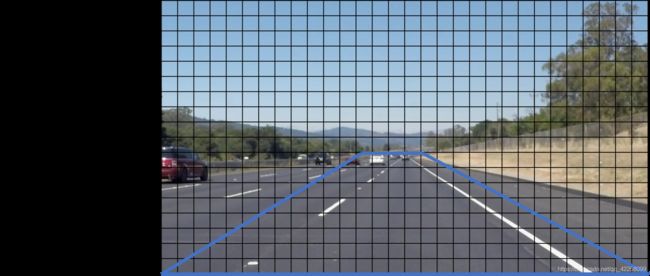
····我们可以看到对于一张图片的二值化处理，除了我们需要的车道信息，还会有周围环境特征，如天空、山、周边荒草环境等，为了提高算法鲁棒性，通过框选感兴趣区域，是一个不错的选择，[masked_edges]即为结果。这里我们只针对单车道线检测，划出图像中关于自身车位的前方及左右半条车道范围延伸至灭点，如上图所示，如针对多车道线测，那在框选时需要更加慎重，除了地平线以上剔除外，地平线以下根据拍摄质量好坏（像素较低时不足以得到一个稳定结果）和有效车道数设定（不要求全检测，只检测左右三车道，更合适用于实车运行）,所用函数见下文代码解析；
····之后就是基于hough变换提取出若干线段，把二值化后的像素坐标点集（X，Y）转化到栅格化的极坐标（r，θ），基于投票选举法，统计得到若干条概率最高的直线，针对这些直线进行合并和剔除，得到最终车道线，如图[line_image]，完工！所用函数见下文代码解析，关于hough变换的具体细节见转载⁵，里面通过图例，直观说明常用图像处理滤波器（转载自其他作者，如有侵权请私戳）

代码讲解

····上面讲解了思路，这里说明一下代码吧。主要是基于每个函数进行讲解，最后再说明优化方向。
详见：https://github.com/wisdom-bob/CarND-LaneLines-P1-master

# importing some useful packages
import matplotlib.pyplot as plt
import matplotlib.image as mpimg
import numpy as np
import math
import cv2

# define some functions
def grayscale(img):
    return cv2.cvtColor(img, cv2.COLOR_RGB2GRAY)
#     return cv2.cvtColor(img, cv2.COLOR_BGR2GRAY) # use BGR2GRAY if you read an image with cv2.imread()
    
def canny(img, low_threshold, high_threshold):
	#  Image Binarization with canny operator
    return cv2.Canny(img, low_threshold, high_threshold)

def gaussian_blur(img, kernel_size):
	#	gaussian filter by (kernel_size,kernel_size) operator
    return cv2.GaussianBlur(img, (kernel_size, kernel_size), 0)

def region_of_interest(img, vertices):
    #defining a blank mask to start with
    mask = np.zeros_like(img)   
    
    #defining a 3 channel or 1 channel color to fill the mask, depending on the input image
    if len(img.shape) > 2:
        channel_count = img.shape[2]  # i.e. 3 or 4 depending on your image
        ignore_mask_color = (255,) * channel_count
    else:
        ignore_mask_color = 255
        
    #filling pixels inside the polygon defined by "vertices" with the fill color    
    cv2.fillPoly(mask, vertices, ignore_mask_color)
    
    #returning the image only where mask pixels are nonzero
    masked_image = cv2.bitwise_and(img, mask)
    return masked_image

def draw_lines(img, lines, color=[255, 0, 0], thickness=8):
    for line in lines:
        for x1,y1,x2,y2 in line:
            cv2.line(img, (x1, y1), (x2, y2), color, thickness)

def Ltopend(arr,imshape):
	#	return the top point(x0,y0) and end point(x1,y1) of the line
    Arr = np.concatenate(arr, axis=0)
    k = sum(Arr[:,1]-Arr[:,3])/sum(Arr[:,0]-Arr[:,2])
    b = Arr[0][1]-k*Arr[0][0]
    
    x0 = int((imshape[0]-b)//k)
    y0 = imshape[0]
    for i in Arr:
        if i[3] == min(min(Arr[:,1]),min(Arr[:,3])):
            x1,y1 = i[3],i[2]
        elif i[1] == min(min(Arr[:,1]),min(Arr[:,3])):
            x1,y1 = i[1],i[0]
    return ((x0,y0),(y1,x1))

def draw_lines2(img, lines, color=[255, 0, 0], thickness=14):
	# updated draw_lines function
    le,ri= [],[]
    for line in lines:
        for x1,y1,x2,y2 in line:
            if (y2-y1)/(x2-x1)<0:
                le.append(line)
            else:
                ri.append(line)
    le = np.array(le)
    ri = np.array(ri)
    points = Ltopend(le,img.shape)
    cv2.line(img, points[0], points[1], color, thickness)
    points = Ltopend(ri,img.shape)
    cv2.line(img, points[0], points[1], color, thickness)    
            
def hough_lines(img, rho, theta, threshold, min_line_len, max_line_gap,flag=0):
	#	according to the HoughLinesP to get the lines, then draw them
    lines = cv2.HoughLinesP(img, rho, theta, threshold, np.array([]), minLineLength=min_line_len, maxLineGap=max_line_gap)
    line_img = np.zeros((img.shape[0], img.shape[1], 3), dtype=np.uint8)
    if flag:
        draw_lines2(line_img, lines, img.shape)
    else:
        draw_lines(line_img, lines)
    return line_img

def weighted_img(img, initial_img, α=0.8, β=1., γ=0.):
	#	image blending
    return cv2.addWeighted(initial_img, α, img, β, γ)

····通过以上函数，我们设置了若干个函数接口用于接入灰度化、高斯滤波、canny二值化、hough变换等，那么基于以上函数，我们可以自己先尝试得到图像处理结果（上图的结果）。

def showimg(subplace, title, _img):
	#	design a subplot_imshow funciton
    plt.subplot(*subplace)
    plt.title(title)
    if len(_img.shape) == 3:
        plt.imshow(_img)
    else:
        plt.imshow(_img, cmap='gray')

#	from loca upload some images
names = []
for file in os.listdir("test_images/"):
    names.append(str(file[:file.rfind('.')]))
    
#	image->grayscale->gaussian_blur->canny->edges
name = names[1]
image = files[name]
gray = grayscale(image)
blur_gray = gaussian_blur(gray,7)
edges = canny(blur_gray, 50, 150)

#	Next we'll create a masked edges image using cv2.fillPoly() to get the region of interest
mask = np.zeros_like(edges)   
ignore_mask_color = 255   
imshape = image.shape

vertices = np.array([[(0,imshape[0]),(410, 330), (550, 330), (imshape[1],imshape[0])]], dtype=np.int32)
masked_edges = region_of_interest(edges,vertices)

#	Define the Hough transform parameters
rho = 1                             # distance resolution in pixels of the Hough grid
theta = np.pi/180                   # angular resolution in radians of the Hough grid
threshold = 15                      # minimum number of votes (intersections in Hough grid cell)
min_line_length = 25                 # minimum number of pixels making up a line
max_line_gap = 25                   # maximum gap in pixels between connectable line segments
line_image = np.copy(image)*0       # creating a blank to draw lines on

#	Run Hough on edge detected image
line_image = hough_lines(masked_edges, rho, theta, threshold, min_line_length, max_line_gap,flag=1)

#	Create the combined image, show and save it
color_edges = np.dstack((edges, edges, edges)) 
finalimg = weighted_img(line_image,image)
# plt.savefig("out"+name)

#	debug with images to show
plt.figure(figsize=[16, 9])
for i, imgname in enumerate(['image', 'gray', 'blur_gray', 'edges', 'masked_edges','line_image']):
    showimg((2, 3, i+1), imgname, eval(imgname))

····在此基础之上，我们已经基本摸清楚了这些函数的具体用途和使用效果，那么我们可以基于上段函数来构建一个function，写定各参数，实现面向实时的单车道线检测处理。

def process_image(image, ignore_mask_color = 255, rho = 1, theta = np.pi/180, threshold = 15, min_line_length = 25,max_line_gap = 25):
	# gray
    gray = grayscale(image)
    
    # blur_gray
    blur_gray = gaussian_blur(gray,7)
    
    # edges
    edges = canny(blur_gray, 50, 150) 
    
    # region-of-interest
    imshape = image.shape
    mask = np.zeros_like(edges)   
    vertices = np.array([[(0,imshape[0]),(410, 330), (550, 330), (imshape[1],imshape[0])]], dtype=np.int32)
    masked_edges = region_of_interest(edges,vertices)

	# creating a blank to draw lines on
    line_image = np.copy(image)*0       

    # Run Hough on edge detected image
    line_image = hough_lines(masked_edges, rho, theta, threshold, min_line_length, max_line_gap,flag=0)

    # Create the combined image, show and save it
    color_edges = np.dstack((edges, edges, edges)) 
    finalimg = weighted_img(line_image,image)
    return finalimg

····此时接入视频，查看结果.

# Import everything needed to edit/save/watch video clips
from moviepy.editor import VideoFileClip
from IPython.display import HTML

white_output = 'test_videos_output/solidWhiteRight.mp4'
clip1 = VideoFileClip("test_videos/solidWhiteRight.mp4")
white_clip = clip1.fl_image(process_image) #NOTE: this function expects color images!!
%time white_clip.write_videofile(white_output, audio=False)

总结和拓展

····至此基于hough的单车道线检测已经完成了，无需gpu，只在cpu上跑可以达到40帧/s，满足实时性要求，算是非常好的结果，而且车道线检测结果非常稳定，只是偶尔会有错帧，而且hough变换只能基于直线来进行，弯道检测必须用其他方法。
····从优化角度去考虑，至少可以再加个平滑器，这样图像效果更棒，提高鲁棒性，不易受偶尔的错帧影响；无法应对复杂场景，可以考虑增加灭点特征，可以减少部分错误结果，提高算法鲁棒性；可以考虑增加跟踪器，提高算法结果的可靠性。
····快去试试吧~~

如有侵权，请私戳~~感谢。

---

1. https://www.cnblogs.com/finlay/p/3665302.html ↩︎

2. https://blog.csdn.net/eastmount/article/details/82216380 ↩︎

3. https://www.cnblogs.com/techyan1990/p/7291771.html ↩︎

4. https://www.cnblogs.com/wlzy/p/7283579.html ↩︎

5. https://blog.csdn.net/yuyuntan/article/details/80141392 ↩︎