【手把手机器学习入门到放弃】SVM支持向量机

支持向量机

打仗的时候只有站最前面的人在打而已

支持向量机也是完成分类问题的一个工具，不同于逻辑回归，在支持向量机解决的分类问题中，只有最靠近对方阵营的样本对分界线的确定起到作用，而远离分界线的那些样本对分界线的确定没有作用。在这样的机制下，SVM拥有更好的鲁棒性，受离群点的影响几乎可忽略不计。

本次演示使用美国成人收入统计模型
数据说明如下：

• age: continuous.
• workclass: Private, Self-emp-not-inc, Self-emp-inc, Federal-gov, Local-gov, State-gov, Without-pay, Never-worked.
• fnlwgt: continuous.
• education: Bachelors, Some-college, 11th, HS-grad, Prof-school, Assoc-acdm, Assoc-voc, 9th, 7th-8th, 12th, Masters, 1st-4th, 10th, Doctorate, 5th-6th, Preschool.
• education-num: continuous.
• marital-status: Married-civ-spouse, Divorced, Never-married, Separated, Widowed, Married-spouse-absent, Married-AF-spouse.
• occupation: Tech-support, Craft-repair, Other-service, Sales, Exec-managerial, Prof-specialty, Handlers-cleaners, Machine-op-inspct, Adm-clerical, Farming-fishing, Transport-moving, Priv-house-serv, Protective-serv, Armed-Forces.
• relationship: Wife, Own-child, Husband, Not-in-family, Other-relative, Unmarried.
• race: White, Asian-Pac-Islander, Amer-Indian-Eskimo, Other, Black.
• sex: Female, Male.
• capital-gain: continuous.
• capital-loss: continuous.
• hours-per-week: continuous.
• native-country: United-States, Cambodia, England, Puerto-Rico, Canada, Germany, Outlying-US(Guam-USVI-etc), India, Japan, Greece, South, China, Cuba, Iran, Honduras, Philippines, Italy, Poland, Jamaica, Vietnam, Mexico, Portugal, Ireland, France, Dominican-Republic, Laos, Ecuador, Taiwan, Haiti, Columbia, Hungary, Guatemala, Nicaragua, Scotland, Thailand, Yugoslavia, El-Salvador, Trinadad&Tobago, Peru, Hong, Holand-Netherlands.

标签有两种：>50K, <=50K.

import pandas as pd 
import numpy as np
from sklearn import svm
import matplotlib.pyplot as plt
import seaborn as sns
from sklearn.model_selection import train_test_split

1. 数据初探

dataframe = pd.read_table('datasets/Adult/adult.data',sep=',',header=None)
dataframe.columns=["age", "workclass", "fnlwgt", "education", "education-num", "marital-status", 
                   "occupation", "relationship", "race", "sex", "capital-gain", "capital-loss", 
                   "hours-per-week", "native-country","salary"]
dataframe.head(3)

/Users/yaochenli/anaconda3/lib/python3.7/site-packages/ipykernel_launcher.py:1: FutureWarning: read_table is deprecated, use read_csv instead.
  """Entry point for launching an IPython kernel.

	age	workclass	fnlwgt	education	education-num	marital-status	occupation	relationship	race	sex	capital-gain	capital-loss	hours-per-week	native-country	salary
0	39	State-gov	77516	Bachelors	13	Never-married	Adm-clerical	Not-in-family	White	Male	2174	0	40	United-States	<=50K
1	50	Self-emp-not-inc	83311	Bachelors	13	Married-civ-spouse	Exec-managerial	Husband	White	Male	0	0	13	United-States	<=50K
2	38	Private	215646	HS-grad	9	Divorced	Handlers-cleaners	Not-in-family	White	Male	0	0	40	United-States	<=50K

2. 缺失值处理

dataframe.workclass.unique()

可以看到这个原始数据里面的缺失值是用“？”表示的

dataframe.shape

(32561, 15)

(dataframe==" ?").sum()

/Users/yaochenli/anaconda3/lib/python3.7/site-packages/pandas/core/ops.py:1649: FutureWarning: elementwise comparison failed; returning scalar instead, but in the future will perform elementwise comparison
  result = method(y)





age                  0
workclass         1836
fnlwgt               0
education            0
education-num        0
marital-status       0
occupation        1843
relationship         0
race                 0
sex                  0
capital-gain         0
capital-loss         0
hours-per-week       0
native-country     583
salary               0
dtype: int64

对比样本量，缺失值不算很多，由于缺失的值都不是标量，而是标签变量，所以我们根据分布进行填充

• 工作类别 workclass

dataframe.workclass.value_counts()

 Private             22696
 Self-emp-not-inc     2541
 Local-gov            2093
 ?                    1836
 State-gov            1298
 Self-emp-inc         1116
 Federal-gov           960
 Without-pay            14
 Never-worked            7
Name: workclass, dtype: int64

这里private明显占了大多数，我们就把缺失值使用Private填充

dataframe.workclass.replace(" ?", " Private", inplace=True)

dataframe.workclass.value_counts()

 Private             24532
 Self-emp-not-inc     2541
 Local-gov            2093
 State-gov            1298
 Self-emp-inc         1116
 Federal-gov           960
 Without-pay            14
 Never-worked            7
Name: workclass, dtype: int64

• 职业 occupation

dataframe.occupation.value_counts()

 Prof-specialty       4140
 Craft-repair         4099
 Exec-managerial      4066
 Adm-clerical         3770
 Sales                3650
 Other-service        3295
 Machine-op-inspct    2002
 ?                    1843
 Transport-moving     1597
 Handlers-cleaners    1370
 Farming-fishing       994
 Tech-support          928
 Protective-serv       649
 Priv-house-serv       149
 Armed-Forces            9
Name: occupation, dtype: int64

这里分布比较平均，我们把“？”单独以Others替代

dataframe.occupation.replace(" ?", " Other", inplace=True)

dataframe.occupation.value_counts()

 Prof-specialty       4140
 Craft-repair         4099
 Exec-managerial      4066
 Adm-clerical         3770
 Sales                3650
 Other-service        3295
 Machine-op-inspct    2002
 Other                1843
 Transport-moving     1597
 Handlers-cleaners    1370
 Farming-fishing       994
 Tech-support          928
 Protective-serv       649
 Priv-house-serv       149
 Armed-Forces            9
Name: occupation, dtype: int64

• 原国籍 native-country

dataframe["native-country"].value_counts()

 United-States                 29170
 Mexico                          643
 ?                               583
 Philippines                     198
 Germany                         137
 Canada                          121
 Puerto-Rico                     114
 El-Salvador                     106
 India                           100
 Cuba                             95
 England                          90
 Jamaica                          81
 South                            80
 China                            75
 Italy                            73
 Dominican-Republic               70
 Vietnam                          67
 Guatemala                        64
 Japan                            62
 Poland                           60
 Columbia                         59
 Taiwan                           51
 Haiti                            44
 Iran                             43
 Portugal                         37
 Nicaragua                        34
 Peru                             31
 Greece                           29
 France                           29
 Ecuador                          28
 Ireland                          24
 Hong                             20
 Trinadad&Tobago                  19
 Cambodia                         19
 Thailand                         18
 Laos                             18
 Yugoslavia                       16
 Outlying-US(Guam-USVI-etc)       14
 Hungary                          13
 Honduras                         13
 Scotland                         12
 Holand-Netherlands                1
Name: native-country, dtype: int64

这里美国的样本量占了绝大多数，我们先使用美国来填充缺失值

dataframe["native-country"].replace(" ?", " United-States", inplace=True)

dataframe["native-country"].value_counts()

 United-States                 29753
 Mexico                          643
 Philippines                     198
 Germany                         137
 Canada                          121
 Puerto-Rico                     114
 El-Salvador                     106
 India                           100
 Cuba                             95
 England                          90
 Jamaica                          81
 South                            80
 China                            75
 Italy                            73
 Dominican-Republic               70
 Vietnam                          67
 Guatemala                        64
 Japan                            62
 Poland                           60
 Columbia                         59
 Taiwan                           51
 Haiti                            44
 Iran                             43
 Portugal                         37
 Nicaragua                        34
 Peru                             31
 France                           29
 Greece                           29
 Ecuador                          28
 Ireland                          24
 Hong                             20
 Cambodia                         19
 Trinadad&Tobago                  19
 Laos                             18
 Thailand                         18
 Yugoslavia                       16
 Outlying-US(Guam-USVI-etc)       14
 Honduras                         13
 Hungary                          13
 Scotland                         12
 Holand-Netherlands                1
Name: native-country, dtype: int64

3. 数据分布初探

1. 探究正负样本的数量关系

plt.figure(figsize=(8,5))
sns.color_palette("Set3")
# sns.set(style="whitegrid")
sns.countplot(dataframe.salary, palette="rocket")
plt.title("distribution of salary")

Text(0.5, 1.0, 'distribution of salary')

可以看到样本标签不是很平衡，但我们用SVM问题不大

1. 探究学历与工资之间的关系

plt.figure(figsize=(20,10))
#sns.set(style="whitegrid")
sns.set()
plt.title("countgrid of education level over salary")
plt.subplot(121)
sns.countplot(x="education", data=dataframe[dataframe["salary"]==" <=50K"], palette="rocket")
plt.xlabel("<=50K")
plt.xticks(rotation=45)
plt.subplot(122)
sns.countplot(x="education", data=dataframe[dataframe["salary"]==" >50K"], palette="rocket")
plt.xlabel(">50K")
plt.xticks(rotation=45)
# plt.legend(loc="upper right")

(array([ 0,  1,  2,  3,  4,  5,  6,  7,  8,  9, 10, 11, 12, 13, 14]),
 )

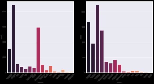
从上面的结果可以看到工资<=50K的人群中，HS-grad，和一些社区学校毕业的居多，而在工资>50K的人群中Bachelor最多

2. 探究年龄与工资之间的关系

plt.figure(figsize=(20,15))
sns.kdeplot(dataframe[dataframe["salary"]==" <=50K"].age, shade=True)
sns.kdeplot(dataframe[dataframe["salary"]==" >50K"].age, shade=True)
plt.legend(["<=50K",">50K"])
plt.title("age distribution over salary")

Text(0.5, 1.0, 'age distribution over salary')

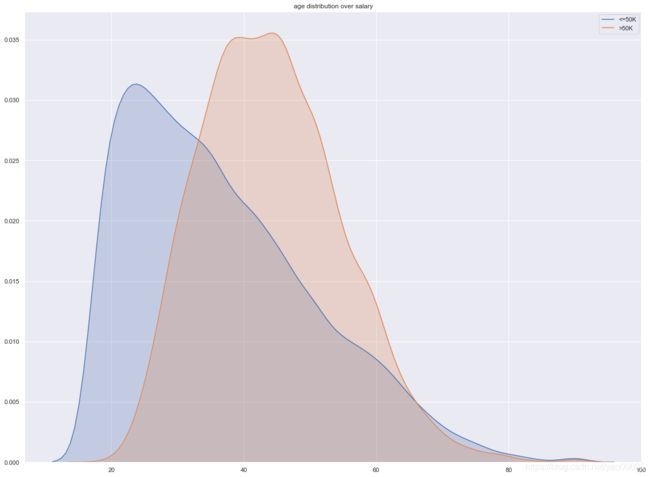
我们可以看到工资较高的人群平均年龄也较高，超过40岁，而工资较低的人群年龄平均在20多。这个是符合我们的预期的

3. 探究性别对工资的影响

plt.figure(figsize=(20,10))
#sns.set(style="whitegrid")
sns.set()
plt.title("countgrid of gender over salary")
plt.subplot(121)
sns.countplot(x="sex", data=dataframe[dataframe["salary"]==" <=50K"], palette="rocket")
plt.xlabel("<=50K")
plt.subplot(122)
sns.countplot(x="sex", data=dataframe[dataframe["salary"]==" >50K"], palette="rocket")
plt.xlabel(">50K")

Text(0.5, 0, '>50K')

可以看到在工资较低的人群中，男女比例大概在5:3，而在工资较高的人群中，男女比大约在5.5:1，看来在高端职业上，美国的职场性别歧视也是十分明显。

4. 探究高工资人群和低工资人群的工作时长

plt.figure(figsize=(20,15))
sns.set()
sns.distplot(dataframe[dataframe["salary"]==" <=50K"]["hours-per-week"],vertical=True)
sns.distplot(dataframe[dataframe["salary"]==" >50K"]["hours-per-week"],vertical=True)
plt.legend(["<=50K",">50K"])
plt.title("age distribution over salary")

Text(0.5, 1.0, 'age distribution over salary')

可以看到普遍来说，工资较低人群每周工作时长比较低，而工资较高的人群确实工作时长也比较高，能者多劳，看来在哪都是这样

5. 探究年龄和工作时长之间的关系 （这个跟模型没关系，纯属满足本人好奇心）

plt.figure(figsize=(15,8))
cmap = sns.cubehelix_palette(rot=-.2, as_cmap=True)
ax = sns.scatterplot(x="age", y="hours-per-week",
                     hue="salary",
                     data=dataframe)

[外链图片转存失败,源站可能有防盗链机制,建议将图片保存下来直接上传(img-VRrp3mtE-1572353712274)(output_42_0.png)]

60岁之后工作时长是明显随着年龄减少的，工资较高人群工作时长集中在40-60小时每周，工作年龄在30岁到60岁，而低工资人群工作时长各种都有。可以推理高工资人群大多数都是坐办公室的，而且基本上也都得加班

4. 建立模型输入

# 对标记变量转换成哑变量 使用pd.get_dummies方法，将salary转换成 <=50K：0，>50K:1
X = dataframe.join(pd.get_dummies(dataframe.loc[:,["workclass","education","occupation","marital-status","relationship",
                                           "race","sex","native-country"]]))
X=X.drop(["workclass","education","marital-status","occupation","relationship",
                                           "race","sex","native-country"], axis=1)
X.salary.replace(" <=50K",0,inplace=True)
X.salary.replace(" >50K",1,inplace=True)
X.head(3)

	age	fnlwgt	education-num	capital-gain	capital-loss	hours-per-week	salary	workclass_ Federal-gov	workclass_ Local-gov	workclass_ Never-worked	...	native-country_ Portugal	native-country_ Puerto-Rico	native-country_ Scotland	native-country_ South	native-country_ Taiwan	native-country_ Thailand	native-country_ Trinadad&Tobago	native-country_ United-States	native-country_ Vietnam	native-country_ Yugoslavia
0	39	77516	13	2174	0	40	0	0	0	0	...	0	0	0	0	0	0	0	1	0	0
1	50	83311	13	0	0	13	0	0	0	0	...	0	0	0	0	0	0	0	1	0	0
2	38	215646	9	0	0	40	0	0	0	0	...	0	0	0	0	0	0	0	1	0	0

3 rows × 107 columns

y=X.salary
X=X.drop(["salary"], axis=1)

X_train, X_test, y_train, y_test = train_test_split(X,y)

X_train.head(3)

	age	fnlwgt	education-num	capital-gain	capital-loss	hours-per-week	workclass_ Federal-gov	workclass_ Local-gov	workclass_ Never-worked	workclass_ Private	...	native-country_ Portugal	native-country_ Puerto-Rico	native-country_ Scotland	native-country_ South	native-country_ Taiwan	native-country_ Thailand	native-country_ Trinadad&Tobago	native-country_ United-States	native-country_ Vietnam	native-country_ Yugoslavia
16834	26	131686	13	0	0	40	0	0	0	1	...	0	0	0	0	0	0	0	1	0	0
14311	33	136331	9	0	0	50	0	0	0	1	...	0	0	0	0	0	0	0	1	0	0
32421	31	298995	9	0	0	35	0	0	0	1	...	0	0	0	0	0	0	0	1	0	0

3 rows × 106 columns

5. 进行模型训练

sklearn里面的SVM模块中分类器当中自带4种核函数（什么是核函数麻烦读者自行百度），分别是：

• 线性核 linear: $(X,X^{\prime })$
• 多项式核 polynomial: $(\gamma <X+X^{\prime }>+r{)}^d$
• 高斯核 rbf $exp(-\gamma ||X-X^{\prime }|{|}^2)$
• sigmoid核 $tanh(\gamma <X,X^{\prime }>+r)$

此外还可以使用自定义的核函数，详见官网：https://scikit-learn.org/stable/auto_examples/svm/plot_custom_kernel.html#sphx-glr-auto-examples-svm-plot-custom-kernel-py

下面我们尝试用4种核函数分别进行训练

1. 线性核

help(svm.SVC)

Help on class SVC in module sklearn.svm.classes:

class SVC(sklearn.svm.base.BaseSVC)
 |  SVC(C=1.0, kernel='rbf', degree=3, gamma='auto_deprecated', coef0=0.0, shrinking=True, probability=False, tol=0.001, cache_size=200, class_weight=None, verbose=False, max_iter=-1, decision_function_shape='ovr', random_state=None)
 |  
 |  C-Support Vector Classification.
 |  
 |  The implementation is based on libsvm. The fit time scales at least
 |  quadratically with the number of samples and may be impractical
 |  beyond tens of thousands of samples. For large datasets
 |  consider using :class:`sklearn.linear_model.LinearSVC` or
 |  :class:`sklearn.linear_model.SGDClassifier` instead, possibly after a
 |  :class:`sklearn.kernel_approximation.Nystroem` transformer.
 |  
 |  The multiclass support is handled according to a one-vs-one scheme.
 |  
 |  For details on the precise mathematical formulation of the provided
 |  kernel functions and how `gamma`, `coef0` and `degree` affect each
 |  other, see the corresponding section in the narrative documentation:
 |  :ref:`svm_kernels`.
 |  
 |  Read more in the :ref:`User Guide `.
 |  
 |  Parameters
 |  ----------
 |  C : float, optional (default=1.0)
 |      Penalty parameter C of the error term.
 |  
 |  kernel : string, optional (default='rbf')
 |      Specifies the kernel type to be used in the algorithm.
 |      It must be one of 'linear', 'poly', 'rbf', 'sigmoid', 'precomputed' or
 |      a callable.
 |      If none is given, 'rbf' will be used. If a callable is given it is
 |      used to pre-compute the kernel matrix from data matrices; that matrix
 |      should be an array of shape ``(n_samples, n_samples)``.
 |  
 |  degree : int, optional (default=3)
 |      Degree of the polynomial kernel function ('poly').
 |      Ignored by all other kernels.
 |  
 |  gamma : float, optional (default='auto')
 |      Kernel coefficient for 'rbf', 'poly' and 'sigmoid'.
 |  
 |      Current default is 'auto' which uses 1 / n_features,
 |      if ``gamma='scale'`` is passed then it uses 1 / (n_features * X.var())
 |      as value of gamma. The current default of gamma, 'auto', will change
 |      to 'scale' in version 0.22. 'auto_deprecated', a deprecated version of
 |      'auto' is used as a default indicating that no explicit value of gamma
 |      was passed.
 |  
 |  coef0 : float, optional (default=0.0)
 |      Independent term in kernel function.
 |      It is only significant in 'poly' and 'sigmoid'.
 |  
 |  shrinking : boolean, optional (default=True)
 |      Whether to use the shrinking heuristic.
 |  
 |  probability : boolean, optional (default=False)
 |      Whether to enable probability estimates. This must be enabled prior
 |      to calling `fit`, and will slow down that method.
 |  
 |  tol : float, optional (default=1e-3)
 |      Tolerance for stopping criterion.
 |  
 |  cache_size : float, optional
 |      Specify the size of the kernel cache (in MB).
 |  
 |  class_weight : {dict, 'balanced'}, optional
 |      Set the parameter C of class i to class_weight[i]*C for
 |      SVC. If not given, all classes are supposed to have
 |      weight one.
 |      The "balanced" mode uses the values of y to automatically adjust
 |      weights inversely proportional to class frequencies in the input data
 |      as ``n_samples / (n_classes * np.bincount(y))``
 |  
 |  verbose : bool, default: False
 |      Enable verbose output. Note that this setting takes advantage of a
 |      per-process runtime setting in libsvm that, if enabled, may not work
 |      properly in a multithreaded context.
 |  
 |  max_iter : int, optional (default=-1)
 |      Hard limit on iterations within solver, or -1 for no limit.
 |  
 |  decision_function_shape : 'ovo', 'ovr', default='ovr'
 |      Whether to return a one-vs-rest ('ovr') decision function of shape
 |      (n_samples, n_classes) as all other classifiers, or the original
 |      one-vs-one ('ovo') decision function of libsvm which has shape
 |      (n_samples, n_classes * (n_classes - 1) / 2). However, one-vs-one
 |      ('ovo') is always used as multi-class strategy.
 |  
 |      .. versionchanged:: 0.19
 |          decision_function_shape is 'ovr' by default.
 |  
 |      .. versionadded:: 0.17
 |         *decision_function_shape='ovr'* is recommended.
 |  
 |      .. versionchanged:: 0.17
 |         Deprecated *decision_function_shape='ovo' and None*.
 |  
 |  random_state : int, RandomState instance or None, optional (default=None)
 |      The seed of the pseudo random number generator used when shuffling
 |      the data for probability estimates. If int, random_state is the
 |      seed used by the random number generator; If RandomState instance,
 |      random_state is the random number generator; If None, the random
 |      number generator is the RandomState instance used by `np.random`.
 |  
 |  Attributes
 |  ----------
 |  support_ : array-like, shape = [n_SV]
 |      Indices of support vectors.
 |  
 |  support_vectors_ : array-like, shape = [n_SV, n_features]
 |      Support vectors.
 |  
 |  n_support_ : array-like, dtype=int32, shape = [n_class]
 |      Number of support vectors for each class.
 |  
 |  dual_coef_ : array, shape = [n_class-1, n_SV]
 |      Coefficients of the support vector in the decision function.
 |      For multiclass, coefficient for all 1-vs-1 classifiers.
 |      The layout of the coefficients in the multiclass case is somewhat
 |      non-trivial. See the section about multi-class classification in the
 |      SVM section of the User Guide for details.
 |  
 |  coef_ : array, shape = [n_class * (n_class-1) / 2, n_features]
 |      Weights assigned to the features (coefficients in the primal
 |      problem). This is only available in the case of a linear kernel.
 |  
 |      `coef_` is a readonly property derived from `dual_coef_` and
 |      `support_vectors_`.
 |  
 |  intercept_ : array, shape = [n_class * (n_class-1) / 2]
 |      Constants in decision function.
 |  
 |  fit_status_ : int
 |      0 if correctly fitted, 1 otherwise (will raise warning)
 |  
 |  probA_ : array, shape = [n_class * (n_class-1) / 2]
 |  probB_ : array, shape = [n_class * (n_class-1) / 2]
 |      If probability=True, the parameters learned in Platt scaling to
 |      produce probability estimates from decision values. If
 |      probability=False, an empty array. Platt scaling uses the logistic
 |      function
 |      ``1 / (1 + exp(decision_value * probA_ + probB_))``
 |      where ``probA_`` and ``probB_`` are learned from the dataset [2]_. For
 |      more information on the multiclass case and training procedure see
 |      section 8 of [1]_.
 |  
 |  Examples
 |  --------
 |  >>> import numpy as np
 |  >>> X = np.array([[-1, -1], [-2, -1], [1, 1], [2, 1]])
 |  >>> y = np.array([1, 1, 2, 2])
 |  >>> from sklearn.svm import SVC
 |  >>> clf = SVC(gamma='auto')
 |  >>> clf.fit(X, y) #doctest: +NORMALIZE_WHITESPACE
 |  SVC(C=1.0, cache_size=200, class_weight=None, coef0=0.0,
 |      decision_function_shape='ovr', degree=3, gamma='auto', kernel='rbf',
 |      max_iter=-1, probability=False, random_state=None, shrinking=True,
 |      tol=0.001, verbose=False)
 |  >>> print(clf.predict([[-0.8, -1]]))
 |  [1]
 |  
 |  See also
 |  --------
 |  SVR
 |      Support Vector Machine for Regression implemented using libsvm.
 |  
 |  LinearSVC
 |      Scalable Linear Support Vector Machine for classification
 |      implemented using liblinear. Check the See also section of
 |      LinearSVC for more comparison element.
 |  
 |  References
 |  ----------
 |  .. [1] `LIBSVM: A Library for Support Vector Machines
 |      `_
 |  
 |  .. [2] `Platt, John (1999). "Probabilistic outputs for support vector
 |      machines and comparison to regularizedlikelihood methods."
 |      `_
 |  
 |  Method resolution order:
 |      SVC
 |      sklearn.svm.base.BaseSVC
 |      sklearn.svm.base.BaseLibSVM
 |      sklearn.base.BaseEstimator
 |      sklearn.base.ClassifierMixin
 |      builtins.object
 |  
 |  Methods defined here:
 |  
 |  __init__(self, C=1.0, kernel='rbf', degree=3, gamma='auto_deprecated', coef0=0.0, shrinking=True, probability=False, tol=0.001, cache_size=200, class_weight=None, verbose=False, max_iter=-1, decision_function_shape='ovr', random_state=None)
 |      Initialize self.  See help(type(self)) for accurate signature.
 |  
 |  ----------------------------------------------------------------------
 |  Data and other attributes defined here:
 |  
 |  __abstractmethods__ = frozenset()
 |  
 |  ----------------------------------------------------------------------
 |  Methods inherited from sklearn.svm.base.BaseSVC:
 |  
 |  decision_function(self, X)
 |      Evaluates the decision function for the samples in X.
 |      
 |      Parameters
 |      ----------
 |      X : array-like, shape (n_samples, n_features)
 |      
 |      Returns
 |      -------
 |      X : array-like, shape (n_samples, n_classes * (n_classes-1) / 2)
 |          Returns the decision function of the sample for each class
 |          in the model.
 |          If decision_function_shape='ovr', the shape is (n_samples,
 |          n_classes).
 |      
 |      Notes
 |      -----
 |      If decision_function_shape='ovo', the function values are proportional
 |      to the distance of the samples X to the separating hyperplane. If the
 |      exact distances are required, divide the function values by the norm of
 |      the weight vector (``coef_``). See also `this question
 |      `_ for further details.
 |      If decision_function_shape='ovr', the decision function is a monotonic
 |      transformation of ovo decision function.
 |  
 |  predict(self, X)
 |      Perform classification on samples in X.
 |      
 |      For an one-class model, +1 or -1 is returned.
 |      
 |      Parameters
 |      ----------
 |      X : {array-like, sparse matrix}, shape (n_samples, n_features)
 |          For kernel="precomputed", the expected shape of X is
 |          [n_samples_test, n_samples_train]
 |      
 |      Returns
 |      -------
 |      y_pred : array, shape (n_samples,)
 |          Class labels for samples in X.
 |  
 |  ----------------------------------------------------------------------
 |  Data descriptors inherited from sklearn.svm.base.BaseSVC:
 |  
 |  predict_log_proba
 |      Compute log probabilities of possible outcomes for samples in X.
 |      
 |      The model need to have probability information computed at training
 |      time: fit with attribute `probability` set to True.
 |      
 |      Parameters
 |      ----------
 |      X : array-like, shape (n_samples, n_features)
 |          For kernel="precomputed", the expected shape of X is
 |          [n_samples_test, n_samples_train]
 |      
 |      Returns
 |      -------
 |      T : array-like, shape (n_samples, n_classes)
 |          Returns the log-probabilities of the sample for each class in
 |          the model. The columns correspond to the classes in sorted
 |          order, as they appear in the attribute `classes_`.
 |      
 |      Notes
 |      -----
 |      The probability model is created using cross validation, so
 |      the results can be slightly different than those obtained by
 |      predict. Also, it will produce meaningless results on very small
 |      datasets.
 |  
 |  predict_proba
 |      Compute probabilities of possible outcomes for samples in X.
 |      
 |      The model need to have probability information computed at training
 |      time: fit with attribute `probability` set to True.
 |      
 |      Parameters
 |      ----------
 |      X : array-like, shape (n_samples, n_features)
 |          For kernel="precomputed", the expected shape of X is
 |          [n_samples_test, n_samples_train]
 |      
 |      Returns
 |      -------
 |      T : array-like, shape (n_samples, n_classes)
 |          Returns the probability of the sample for each class in
 |          the model. The columns correspond to the classes in sorted
 |          order, as they appear in the attribute `classes_`.
 |      
 |      Notes
 |      -----
 |      The probability model is created using cross validation, so
 |      the results can be slightly different than those obtained by
 |      predict. Also, it will produce meaningless results on very small
 |      datasets.
 |  
 |  ----------------------------------------------------------------------
 |  Methods inherited from sklearn.svm.base.BaseLibSVM:
 |  
 |  fit(self, X, y, sample_weight=None)
 |      Fit the SVM model according to the given training data.
 |      
 |      Parameters
 |      ----------
 |      X : {array-like, sparse matrix}, shape (n_samples, n_features)
 |          Training vectors, where n_samples is the number of samples
 |          and n_features is the number of features.
 |          For kernel="precomputed", the expected shape of X is
 |          (n_samples, n_samples).
 |      
 |      y : array-like, shape (n_samples,)
 |          Target values (class labels in classification, real numbers in
 |          regression)
 |      
 |      sample_weight : array-like, shape (n_samples,)
 |          Per-sample weights. Rescale C per sample. Higher weights
 |          force the classifier to put more emphasis on these points.
 |      
 |      Returns
 |      -------
 |      self : object
 |      
 |      Notes
 |      -----
 |      If X and y are not C-ordered and contiguous arrays of np.float64 and
 |      X is not a scipy.sparse.csr_matrix, X and/or y may be copied.
 |      
 |      If X is a dense array, then the other methods will not support sparse
 |      matrices as input.
 |  
 |  ----------------------------------------------------------------------
 |  Data descriptors inherited from sklearn.svm.base.BaseLibSVM:
 |  
 |  coef_
 |  
 |  ----------------------------------------------------------------------
 |  Methods inherited from sklearn.base.BaseEstimator:
 |  
 |  __getstate__(self)
 |  
 |  __repr__(self, N_CHAR_MAX=700)
 |      Return repr(self).
 |  
 |  __setstate__(self, state)
 |  
 |  get_params(self, deep=True)
 |      Get parameters for this estimator.
 |      
 |      Parameters
 |      ----------
 |      deep : boolean, optional
 |          If True, will return the parameters for this estimator and
 |          contained subobjects that are estimators.
 |      
 |      Returns
 |      -------
 |      params : mapping of string to any
 |          Parameter names mapped to their values.
 |  
 |  set_params(self, **params)
 |      Set the parameters of this estimator.
 |      
 |      The method works on simple estimators as well as on nested objects
 |      (such as pipelines). The latter have parameters of the form
 |      ``__`` so that it's possible to update each
 |      component of a nested object.
 |      
 |      Returns
 |      -------
 |      self
 |  
 |  ----------------------------------------------------------------------
 |  Data descriptors inherited from sklearn.base.BaseEstimator:
 |  
 |  __dict__
 |      dictionary for instance variables (if defined)
 |  
 |  __weakref__
 |      list of weak references to the object (if defined)
 |  
 |  ----------------------------------------------------------------------
 |  Methods inherited from sklearn.base.ClassifierMixin:
 |  
 |  score(self, X, y, sample_weight=None)
 |      Returns the mean accuracy on the given test data and labels.
 |      
 |      In multi-label classification, this is the subset accuracy
 |      which is a harsh metric since you require for each sample that
 |      each label set be correctly predicted.
 |      
 |      Parameters
 |      ----------
 |      X : array-like, shape = (n_samples, n_features)
 |          Test samples.
 |      
 |      y : array-like, shape = (n_samples) or (n_samples, n_outputs)
 |          True labels for X.
 |      
 |      sample_weight : array-like, shape = [n_samples], optional
 |          Sample weights.
 |      
 |      Returns
 |      -------
 |      score : float
 |          Mean accuracy of self.predict(X) wrt. y.

clf = svm.SVC(C=1.0, kernel="linear", verbose=True, max_iter=10000, cache_size=500,class_weight="balanced")
clf.fit(X_train, y_train)

[LibSVM]

SVC(C=1.0, cache_size=500, class_weight='balanced', coef0=0.0,
    decision_function_shape='ovr', degree=3, gamma='auto_deprecated',
    kernel='linear', max_iter=10000, probability=False, random_state=None,
    shrinking=True, tol=0.001, verbose=True)

# 进行预测
y_pred_linear = clf.predict(X_test)

# 查看得分
clf.score(X_test,y_test)

0.7221471563689964

2. 多项式核

clf = svm.SVC(C=1.0, kernel="poly", degree=2, verbose=True, max_iter=10000, cache_size=500,class_weight="balanced")
clf.fit(X_train, y_train)

[LibSVM]
SVC(C=1.0, cache_size=500, class_weight='balanced', coef0=0.0,
    decision_function_shape='ovr', degree=2, gamma='auto_deprecated',
    kernel='poly', max_iter=10000, probability=False, random_state=None,
    shrinking=True, tol=0.001, verbose=True)

y_pred_poly = clf.predict(X_test)

clf.score(X_test,y_test)

0.7419235966097532

得分比线性核高了不少

3. 高斯核

clf = svm.SVC(C=1.0, kernel="rbf", verbose=True, gamma='auto', max_iter=10000, cache_size=1000)
clf.fit(X_train, y_train)

[LibSVM]

SVC(C=1.0, cache_size=1000, class_weight=None, coef0=0.0,
    decision_function_shape='ovr', degree=3, gamma='auto', kernel='rbf',
    max_iter=10000, probability=False, random_state=None, shrinking=True,
    tol=0.001, verbose=True)

y_pred_rbf = clf.predict(X_test)

clf.score(X_test,y_test)

0.7531015845719199

4. sigmoid核

clf = svm.SVC(C=1.0, kernel="sigmoid", verbose=True, max_iter=10000, cache_size=500)
clf.fit(X_train, y_train)

[LibSVM]
SVC(C=1.0, cache_size=500, class_weight=None, coef0=0.0,
    decision_function_shape='ovr', degree=3, gamma='auto_deprecated',
    kernel='sigmoid', max_iter=10000, probability=False, random_state=None,
    shrinking=True, tol=0.001, verbose=True)

y_pred_sigmoid = clf.predict(X_test)

clf.score(X_test,y_test)

0.7592433361994841

在都运行10000此迭代的情况下，除了线性核表现较差之外，其他三个核的表现都差不多

我们下面实验一下四种核的收敛速度

iter_num=[x for x in range(1000,11000,1000)]

linear=[]
poly=[]
rbf=[]
sigmoid=[]
for iters in iter_num:
    clf1 = svm.SVC(C=1.0, kernel="linear", max_iter=iters, cache_size=500)
    clf1.fit(X_train, y_train)
    linear.append(clf1.score(X_test,y_test))
    
    clf2 = svm.SVC(C=1.0, kernel="poly", degree=2, max_iter=iters, cache_size=500)
    clf2.fit(X_train, y_train)
    poly.append(clf2.score(X_test,y_test))
    
    clf3 = svm.SVC(C=0.1, kernel="rbf", gamma='scale', max_iter=iters, cache_size=500)
    clf3.fit(X_train,y_train)
    rbf.append(clf3.score(X_test,y_test))
    
    clf4 = svm.SVC(C=1.0, kernel="sigmoid", max_iter=iters, cache_size=500)
    clf4.fit(X_train,y_train)
    sigmoid.append(clf4.score(X_test,y_test))
    print(iters)

ax=plt.figure(figsize=(15,8))
data = pd.DataFrame({"linear":linear,"poly":poly, "rbf": rbf, "sigmoid": sigmoid},index=iter_num)
sns.lineplot(data=data, palette="tab10", linewidth=2.5)
plt.xlabel("rounds")
plt.ylabel("score")
plt.xticks(iter_num)
plt.title("score variation over rounds of four kinds of kernels")

Text(0.5, 1.0, 'score variation over rounds of four kinds of kernels')

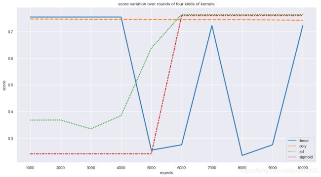
可以看到线性核和多项式核收敛的比较快，在1000轮以前已经收敛,随着轮数增加线性核反而出现了震荡，而高斯核和sigmoid核收敛的较慢，在5000到6000轮之间收敛了。为了不摧残笔者的电脑了就不做更细粒度的分析了。

6. 模型评价

from sklearn import metrics
# 线性核的报告
print(metrics.classification_report(y_test, y_pred_linear))

              precision    recall  f1-score   support

           0       0.76      0.93      0.84      6181
           1       0.21      0.06      0.09      1960

    accuracy                           0.72      8141
   macro avg       0.48      0.49      0.46      8141
weighted avg       0.63      0.72      0.66      8141

# 多项式核的报告
print(metrics.classification_report(y_test, y_pred_poly))

              precision    recall  f1-score   support

           0       0.76      0.97      0.85      6181
           1       0.20      0.02      0.04      1960

    accuracy                           0.74      8141
   macro avg       0.48      0.50      0.45      8141
weighted avg       0.62      0.74      0.66      8141

# 高斯核的报告
print(metrics.classification_report(y_test, y_pred_rbf))

              precision    recall  f1-score   support

           0       0.77      0.97      0.86      6181
           1       0.42      0.07      0.12      1960

    accuracy                           0.75      8141
   macro avg       0.59      0.52      0.49      8141
weighted avg       0.68      0.75      0.68      8141

# sigmoid核的报告
print(metrics.classification_report(y_test, y_pred_sigmoid))

              precision    recall  f1-score   support

           0       0.76      1.00      0.86      6181
           1       0.00      0.00      0.00      1960

    accuracy                           0.76      8141
   macro avg       0.38      0.50      0.43      8141
weighted avg       0.58      0.76      0.66      8141

总结一下，SVM是一种将特征投射到高维平面上进行分割的方法，如果使用rbf核，则可以切割出任意弯曲的边界。在数据分析中是一种常用的分类器。