【Deep Learning】1.深度学习：稀疏自编码器

最近开始学习深度学习的内容，先介绍下自己的学习背景，本人才学习机器学习不到一个月的时间，是在cousera上Andrew Ng的机器学习的课，花了一个多星期的时间把那门课学完了，感觉算是入门了，但是这肯定不够（因为自己去翻了翻Simon Haykin的《神经网络与机器学习》，发现有好多还是迷迷糊糊的，所以打算再继续学些），然后就想在这方面多学些，看到有人推荐深度学习（Deep Learning）这门课，于是就来学了。巧的是，这门课也是Andrew Ng的，之前在cousera上学到的知识刚好成为了预备知识。别担心知识过不了关，我看的这两门课程都是入门级的。

 

稀疏自编码器（sparsity autoencoder）：

1.介绍

  监督性学习是人工智能当中最强大的工具之一，涉及到智能识别、无人车等等。但是监督性学习在如今还是被严重的限制住了。特别地，大多数监督性学习的应用仍要求人为地指定输入的特征。一旦得到一个好的特征表示，监督性学习通常能够很好的工作，然而在类似于计算机视觉、音频处理和自然语言处理中，成百上千的研究人员用了许多年头手工地在寻找最好的特征。尽管有很多非常机智的方法找到特征，但是人们不得不考虑是否能够做得更好。理想地，我们更希望能够拥有一种自动学习寻找特征的方法。

  这里介绍一种叫稀疏自编码器学习算法。这是一种能够自动从非标号数据中学习特征的方法。更进一步的，还有很多更加复杂的稀疏自编码器学习算法，就不一一介绍了。

  我们先引入监督性学习的前向神经网络和后传播算法。然后介绍如何通过这两个算法构造一个非监督性学习的自编码器。最后我们进一步得到一个稀疏的自编码器。

 

2.神经网络

  先回顾一个最简单的神经元

 

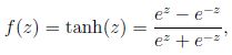其中X1，X2，X3是输入值，而+1是的作用是偏移；然后输出值其中f被称为激活函数，通常有两种表示形式，一种是sigmoid函数1/(1+e^(-Z))，另一种是tanh函数，图像分别如下

，由图可以看出，这两个函数的区别在于sigmoid函数为假时函数值趋于0，为真时函数值趋于1，而tanh函数为假时函数值趋于-1，为真时函数值趋于1，关于tanh函数，在Andrew Ng的machine learning的课上没有提到，所以这里应该是第一次提，不过接下来的内容还是以f为sigmoid函数为主，因此不用担心与machine learning课上的有什么多大的变化。

2.1 神经网络公式化

  还是放出一张图出来，感觉图出来了，就一目了然了

 

我们称L1为输入层，L2为隐藏层，L3为输出层，不包括偏移值+1在内，这个神经网络共有3个输入单元，3个隐藏单元，1个输出单元，其中隐藏单元的激活值a1，a2，a3和偏移值一起与W，b求内积得到下一层的输入z，具体数学公式如下：

 

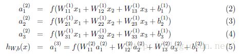
其中，因此

当然神经网络还可以更多的神经元，如

 

不过计算过程还是一样，不用担心。

2.2后传播算法

后传播算法主要用来快速的计算J（W,b）在W和b上的梯度（其实就是导数），用来做梯度下降来得到局部最优的差值，从而得到局部最优的theta，由于这个算法在原教程上也是草草而过，因此我也就把公式放出来吧，有兴趣的大神再去研究，如果有什么好的资源希望能跟小弟我分享下，我后来也尽力会把这些细节弄懂，然后把这部分补充好。

 

 

2.3 梯度检查

上面求梯度的方法很复杂，而且很容易就出错，因此在写完后传播算法后不急着应用，应该用梯度检查的方法检查一下，梯度检查方法很简单，就利用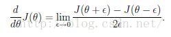，就是求导数的方法。epsilon通常选择e-4。这种方法很简单，但是很慢，速度跟theta的维度有关，如果theta是m维的，J（theta）里面包含一个n次的循环（跟输入集大小有关），每次循环都要过p^2的计算，那么算法复杂度有m*n*p^2这么恐怖（如果有错希望纠正），小数据还是一回事，大数据就呵呵了。因此这也是为什么推荐用后传播算法的原因，对于梯度检查，由于速度慢的问题，我认为没必要对theta中所有的元素的检查，如果你想快点看到结果的话，截取一部分检查就好了。

 

3.自编码器和稀疏性

  截止到目前我们只讨论了监督性学习的神经网络，接着假设我们只有一个无标识训练集，令目标结果集等价于训练集，即，我们就可以得到自编码器神经网络这一个非监督性学习算法（其实用的还是监督性学习那套思路，只不过这次是只有输入集没有结果集，所以我们就让结果集等于目标集了）。

一个自编码器神经网络例子，可以看出与监督性学习的图没什么区别

 

自编码器试图找到一个恒等函数，使得。然而这个函数看起来非常没价值，但如果对隐藏节点加以控制，我们能够发现数据集一些有趣的结构。一个具体的例子，假设输入x是一张10X10的图片的像素点，也即n=100，而只有50个隐藏单元，同时我们要求y=x，也即y也是100维的，对于这样的神经网络，将学到一种对输入的压缩表示。如果输入的x是完全随机的，即彼此不存在联系，那么这个压缩任务将难以进行，但是如果x的特征之间存在某种联系，那么这个算法将有利于找到这部分联系。事实上，简单的自编码器的作用与PCA相似（一种非监督性的降维算法）。

上面的讨论集中在于隐藏单元少的情况，但是即使隐藏单元数量很多（甚至大于输入的特征数），通过对隐藏节点加以限制，我们依旧能够找到数据中有趣的结构。这种限制称为稀疏限制。

  下面给出一些新的记号

   隐藏单元j的平均激活值，以及系数参数，理想地，我们希望。为了实现这一点，我们引入一个新的差值函数（这个函数长得十分像监督性学习中的分类问题的差值函数），记为（），当=0.2时，这个函数的图像是这样的，

发现在=0.2的点处能够取得最小值0

因此，为了能够尽可能实现，我们需要最小化，与之前的差值函数一起考虑，我们可以得到

 

并且在后向传播算法中，我们将使用

 

 

 

可视化自编码器训练结果（这部分我在网上找到翻译版的T T...）：

训练完（稀疏）自编码器，我们还想把这自编码器学到的函数可视化出来，好弄明白它到底学到了什么。我们以在10×10图像（即n=100）上训练自编码器为例。在该自编码器中，每个隐藏单元i对如下关于输入的函数进行计算：

我们将要可视化的函数，就是上面这个以2D图像为输入、并由隐藏单元i计算出来的函数。它是依赖于参数的（暂时忽略偏置项bi）。需要注意的是，可看作输入的非线性特征。不过还有个问题：什么样的输入图像可让得到最大程度的激励？（通俗一点说，隐藏单元要找个什么样的特征？）。这里我们必须给加约束，否则会得到平凡解。若假设输入有范数约束，则可证（请读者自行推导）令隐藏单元得到最大激励的输入应由下面公式计算的像素给出（共需计算100个像素，j=1,…,100）：

当我们用上式算出各像素的值、把它们组成一幅图像、并将图像呈现在我们面前之时，隐藏单元所追寻特征的真正含义也渐渐明朗起来。

假如我们训练的自编码器有100个隐藏单元，可视化结果就会包含100幅这样的图像——每个隐藏单元都对应一幅图像。审视这100幅图像，我们可以试着体会这些隐藏单元学出来的整体效果是什么样的。

当我们对稀疏自编码器（100个隐藏单元，在10X10像素的输入上训练 ）进行上述可视化处理之后，结果如下所示：

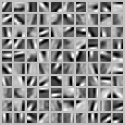
上图的每个小方块都给出了一个（带有有界范数 的）输入图像，它可使这100个隐藏单元中的某一个获得最大激励。我们可以看到，不同的隐藏单元学会了在图像的不同位置和方向进行边缘检测。

显而易见，这些特征对物体识别等计算机视觉任务是十分有用的。若将其用于其他输入域（如音频），该算法也可学到对这些输入域有用的表示或特征。

 

后来发现网上其实有翻译版的，吐血...这是我刚开始写博客，感觉这样自已重新过一遍很多之前漏掉的，还有一些英文版本身的一些错误都发现了，总之没算白写吧。对这部分的如果有什么不清楚或者觉得可以补充的，麻烦各位大神指点，谢谢~

 

练习题：

这次的练习题不算难，不知道后面的会不会难度加大...其实如果有上个Andrew Ng在coursera上开的Machine Learning的课，会发现，这次的作业与那门课的作业有很大的相似之处，有很多甚至都可以照搬的，不过由于是在学习阶段，个人认为还是很有必要自己重新打一遍吧。

工作工具是matlab，有关的作业以及英文教程可以到网站下载：http://deeplearning.stanford.edu/wiki/index.php/UFLDL_Tutorial

中文版的教程：http://deeplearning.stanford.edu/wiki/index.php/UFLDL%E6%95%99%E7%A8%8B

function numgrad = computeNumericalGradient(J, theta)
% numgrad = computeNumericalGradient(J, theta)
% theta: a vector of parameters
% J: a function that outputs a real-number. Calling y = J(theta) will return the
% function value at theta. 
  
% Initialize numgrad with zeros
numgrad = zeros(size(theta));

%% ---------- YOUR CODE HERE --------------------------------------
% Instructions: 
% Implement numerical gradient checking, and return the result in numgrad.  
% (See Section 2.3 of the lecture notes.)
% You should write code so that numgrad(i) is (the numerical approximation to) the 
% partial derivative of J with respect to the i-th input argument, evaluated at theta.  
% I.e., numgrad(i) should be the (approximately) the partial derivative of J with 
% respect to theta(i).
%                
% Hint: You will probably want to compute the elements of numgrad one at a time. 



perturb = zeros(size(theta));
e = 1e-4;
for p = 1:numel(theta),
    % Set perturbation vector
    perturb(p) = e;
    loss1 = J(theta - perturb);
    loss2 = J(theta + perturb);
    % Compute Numerical Gradient
    numgrad(p) = (loss2 - loss1) / (2*e);
    perturb(p) = 0;
end;






%% ---------------------------------------------------------------
end

function patches = sampleIMAGES()
% sampleIMAGES
% Returns 10000 patches for training

load IMAGES;    % load images from disk 

patchsize = 8;  % we'll use 8x8 patches 
numpatches = 10000;

% Initialize patches with zeros.  Your code will fill in this matrix--one
% column per patch, 10000 columns. 
patches = zeros(patchsize*patchsize, numpatches);

%% ---------- YOUR CODE HERE --------------------------------------
%  Instructions: Fill in the variable called "patches" using data 
%  from IMAGES.  
%  
%  IMAGES is a 3D array containing 10 images
%  For instance, IMAGES(:,:,6) is a 512x512 array containing the 6th image,
%  and you can type "imagesc(IMAGES(:,:,6)), colormap gray;" to visualize
%  it. (The contrast on these images look a bit off because they have
%  been preprocessed using using "whitening."  See the lecture notes for
%  more details.) As a second example, IMAGES(21:30,21:30,1) is an image
%  patch corresponding to the pixels in the block (21,21) to (30,30) of
%  Image 1


X = round(1+rand(numpatches,1)*504);
Y = round(1+rand(numpatches,1)*504);
Z = round(1+rand(numpatches,1)*9);

m = patchsize*patchsize;
for i = 1 : numpatches,
    patches(:, i) = reshape(IMAGES(X(i):(X(i)+7), Y(i):(Y(i)+7), Z(i)), m, 1);
end;







%% ---------------------------------------------------------------
% For the autoencoder to work well we need to normalize the data
% Specifically, since the output of the network is bounded between [0,1]
% (due to the sigmoid activation function), we have to make sure 
% the range of pixel values is also bounded between [0,1]
patches = normalizeData(patches);

end


%% ---------------------------------------------------------------
function patches = normalizeData(patches)

% Squash data to [0.1, 0.9] since we use sigmoid as the activation
% function in the output layer

% Remove DC (mean of images). 
patches = bsxfun(@minus, patches, mean(patches));

% Truncate to +/-3 standard deviations and scale to -1 to 1
pstd = 3 * std(patches(:));
patches = max(min(patches, pstd), -pstd) / pstd;

% Rescale from [-1,1] to [0.1,0.9]
patches = (patches + 1) * 0.4 + 0.1;

end

function [cost,grad] = sparseAutoencoderCost(theta, visibleSize, hiddenSize, ...
                                             lambda, sparsityParam, beta, data)

% visibleSize: the number of input units (probably 64) 
% hiddenSize: the number of hidden units (probably 25) 
% lambda: weight decay parameter
% sparsityParam: The desired average activation for the hidden units (denoted in the lecture
%                           notes by the greek alphabet rho, which looks like a lower-case "p").
% beta: weight of sparsity penalty term
% data: Our 64x10000 matrix containing the training data.  So, data(:,i) is the i-th training example. 
  
% The input theta is a vector (because minFunc expects the parameters to be a vector). 
% We first convert theta to the (W1, W2, b1, b2) matrix/vector format, so that this 
% follows the notation convention of the lecture notes. 

W1 = reshape(theta(1:hiddenSize*visibleSize), hiddenSize, visibleSize);
W2 = reshape(theta(hiddenSize*visibleSize+1:2*hiddenSize*visibleSize), visibleSize, hiddenSize);
b1 = theta(2*hiddenSize*visibleSize+1:2*hiddenSize*visibleSize+hiddenSize);
b2 = theta(2*hiddenSize*visibleSize+hiddenSize+1:end);

% Cost and gradient variables (your code needs to compute these values). 
% Here, we initialize them to zeros. 
cost = 0;
W1grad = zeros(size(W1)); 
W2grad = zeros(size(W2));
b1grad = zeros(size(b1)); 
b2grad = zeros(size(b2));

%% ---------- YOUR CODE HERE --------------------------------------
%  Instructions: Compute the cost/optimization objective J_sparse(W,b) for the Sparse Autoencoder,
%                and the corresponding gradients W1grad, W2grad, b1grad, b2grad.
%
% W1grad, W2grad, b1grad and b2grad should be computed using backpropagation.
% Note that W1grad has the same dimensions as W1, b1grad has the same dimensions
% as b1, etc.  Your code should set W1grad to be the partial derivative of J_sparse(W,b) with
% respect to W1.  I.e., W1grad(i,j) should be the partial derivative of J_sparse(W,b) 
% with respect to the input parameter W1(i,j).  Thus, W1grad should be equal to the term 
% [(1/m) \Delta W^{(1)} + \lambda W^{(1)}] in the last block of pseudo-code in Section 2.2 
% of the lecture notes (and similarly for W2grad, b1grad, b2grad).
% 
% Stated differently, if we were using batch gradient descent to optimize the parameters,
% the gradient descent update to W1 would be W1 := W1 - alpha * W1grad, and similarly for W2, b1, b2. 
% 

m = size(data, 2);
Z2 = W1*data+repmat(b1, 1, m);
A2 = sigmoid(Z2);
Z3 = W2*A2+repmat(b2, 1, m);
A3 = sigmoid(Z3);

tmp = A3-data;

sparsityParamTmp = sum(A2, 2)/m;
KLSum = sum(sparsityParam.*log(sparsityParam./sparsityParamTmp)+...
(1-sparsityParam).*log((1-sparsityParam)./(1-sparsityParamTmp)));

cost = sum(sum(tmp.^2))/(2*m);
cost = cost+lambda*sum([W1(:); W2(:)].^2)/2+beta*KLSum;

T3 = tmp.*sigmoidGradient(Z3);
T2 = W2'*T3.*sigmoidGradient(Z2);
T2 = (W2'*T3+repmat(beta.*(-sparsityParam./sparsityParamTmp+(1-sparsityParam)./...
    (1-sparsityParamTmp)), 1, m)).*sigmoidGradient(Z2);
W2grad = (T3*A2')/m;
W2grad = W2grad + lambda*W2;
b2grad = sum(T3, 2)/m;
W1grad = (T2*data')/m;
W1grad = W1grad + lambda*W1;
b1grad = sum(T2, 2)/m;


%-------------------------------------------------------------------
% After computing the cost and gradient, we will convert the gradients back
% to a vector format (suitable for minFunc).  Specifically, we will unroll
% your gradient matrices into a vector.

grad = [W1grad(:) ; W2grad(:) ; b1grad(:) ; b2grad(:)];

end

%-------------------------------------------------------------------
% Here's an implementation of the sigmoid function, which you may find useful
% in your computation of the costs and the gradients.  This inputs a (row or
% column) vector (say (z1, z2, z3)) and returns (f(z1), f(z2), f(z3)). 

function sigm = sigmoid(x)
  
    sigm = 1 ./ (1 + exp(-x));
end
%----------------------------------
这里补充一个我自己的函数
function g = sigmoidGradient(z)
g = sigmoid(z).*(1-sigmoid(z));
end


我的实验结果入下：