数据科学包-Day4-可视化分析（二）

注释

import matplotlib.pyplot as plt
import numpy as np

x = np.arange(-10,11,1)
y=x*x
plt.plot(x,y)
plt.annotate('this is the bottom', xy=(0,1),xytext=(0,20),
             arrowprops=dict(facecolor='r',frac=0.2,headwidth=30,width=10))
plt.show()

文字

import matplotlib.pyplot as plt
import numpy as np

x = np.arange(-10,11,1)
y=x*x
plt.plot(x,y)
plt.text(-2,40,'functio:y=x*x',family='serif')
plt.text(-2,20,'functio:y=x*x',family='fantasy',size=20,color='g',weight='light',bbox=dict(facecolor='r',alpha=0.2))
plt.show()

Tax公式

import matplotlib.pyplot as plt
import numpy as np

fig=plt.figure()
ax=fig.add_subplot(111)
ax.set_xlim([1,7])
ax.set_ylim([1,6])
ax.text(2,4,r"$\alpha \beta_i \lambda \omega $",size=25)
ax.text(4,4,r"$\sin(0)=\cos(\frac{\pi}{2}) $",size=25)
ax.text(2,2,r"$\lim_{x \rightarrow y} \frac{1}{x^3}$",size=25)
ax.text(4,2,r"$ \sqrt[4]{x}=\sqrt{y} $",size=25)
plt.show()

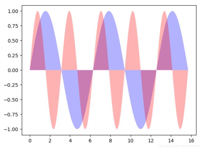
区域填充

import matplotlib.pyplot as plt
import numpy as np

x=np.linspace(0,5*np.pi,1000)
y1=np.sin(x)
y2=np.sin(2*x)

plt.fill(x,y1,'b',alpha=0.3)
plt.fill(x,y2,'r',alpha=0.3)
fig=plt.figure()
ax=plt.gca()
ax.plot(x,y1,x,y2,color='black')
ax.fill_between(x,y1,y2,where=y1>=y2,facecolor='yellow',interpolate=True)
ax.fill_between(x,y1,y2,where=y2>y1,facecolor='green',interpolate=True)
plt.show()

形状

import matplotlib.pyplot as plt
import numpy as np
import matplotlib.patches as mpatches

fig, ax=plt.subplots()
xy1=np.array([0.2,0.2])
xy2=np.array([0.2,0.8])
xy3=np.array([0.8,0.2])
xy4=np.array([0.8,0.8])
circle=mpatches.Circle(xy1,0.05)

ax.add_patch(circle)
rect=mpatches.Rectangle(xy2,0.2,0.1,color='r')
ax.add_patch(rect)
polygon=mpatches.RegularPolygon(xy3,5,0.1,color='g')
ax.add_patch(polygon)
ellipse=mpatches.Ellipse(xy4,0.4,0.2,color='y')
ax.add_patch(ellipse)
plt.axis('equal')
plt.grid()
plt.show()

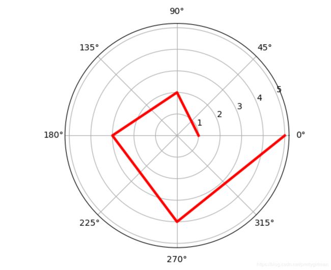
极坐标

import matplotlib.pyplot as plt
import numpy as np
r=np.empty(5)
r.fill(5)
r=np.arange(1,6,1)

theta=[0,np.pi/2,np.pi,3*np.pi/2,2*np.pi]
ax=plt.subplot(111,projection='polar')
ax.plot(theta,r,color='r',linewidth=3)
ax.grid(True)
plt.show()

函数积分图

import matplotlib.pyplot as plt
import numpy as np
from matplotlib.patches import Polygon

def func(x):
    return -(x-2)*(x-8)+40

x=np.linspace(0,10)
y=func(x)
fig, ax=plt.subplots()
plt.plot(x,y,'r',linewidth=1)
a = 2
b = 9
ax.set_xticks([a,b])
ax.set_xticklabels(['$a$','$b$'])
ix=np.linspace(a,b)
iy=func(ix)
ixy=zip(ix,iy)
verts=[(a,0)]+list(ixy)+[(b,0)]
poly=Polygon(verts,facecolor='0.9',edgecolor='0.5')
ax.add_patch(poly)
plt.figtext(0.9,0.05,'$x$')
plt.figtext(0.1,0.9,'$y$')

x_math=(a+b)*0.5
y_math=35
plt.text(x_math,y_math,r'$\int_a^b(-(x-2)*(x-8)+40)dx$',fontsize=13,horizontalalignment='center')
ax.set_yticks([])
plt.show()

散点-条形图

import matplotlib.pyplot as plt
import numpy as np

plt.style.use('ggplot')

x=np.random.randn(200)
y=x+np.random.randn(200)*0.5

margin_border=0.1
width=0.6
margin_between=0.02
height=0.2

left_s=margin_border
bottom_s=margin_border
height_s=width
width_s=width

left_x=margin_border
bottom_x=margin_border+width+margin_between
height_x=height
width_x=width

left_y=margin_border+width+margin_between
bottom_y=margin_border
height_y=width
width_y=height

plt.figure(1,figsize=(8,8))

rect_s=[left_s,bottom_s,width_s,height_s]
rect_x=[left_x,bottom_x,width_x,height_x]
rect_y=[left_y,bottom_y,width_y,height_y]
axScatter=plt.axes(rect_s)
axHisX=plt.axes(rect_x)
axHisY=plt.axes(rect_y)

axHisX.set_xticks([])
axHisY.set_yticks([])

axScatter.scatter(x,y)

bin_width=0.25
xymax=np.max([np.max(np.fabs(x)),np.max(np.fabs(y))])
lim=int(xymax/bin_width+1)*bin_width

axScatter.set_xlim(-lim,lim)
axScatter.set_ylim(-lim,lim)

bins=np.arange(-lim,lim+bin_width,bin_width)

axHisX.hist(x,bins=bins)
axHisY.hist(y,bins=bins,orientation='horizontal')
axHisX.set_xlim(axScatter.get_xlim())
axHisY.set_ylim(axScatter.get_ylim())

plt.title('Scatter and Hist')

plt.show()