python open-cv 基础知识总结(三)
上一章:python open-cv 基础知识总结(二)
1. 轮廓中心计算
本教程的目标是
(1) 检测图像中每个形状的轮廓,
(2) 计算轮廓的中心 -也称为区域的 质心 。
为了实现这些目标,我们需要执行一些图像预处理,包括:
- 转换为灰度
- 进行模糊处理以减少高频噪声,从而使轮廓检测过程更加精确
- 图像的二值化。通常,边缘检测和阈值化用于该过程。在这篇文章中,我们将应用阈值化
# import the necessary packages
import argparse
import imutils
import cv2

# construct the argument parse and parse the arguments
ap = argparse.ArgumentParser()
ap.add_argument("-i", "--image", required=True,
	help="path to the input image")
args = vars(ap.parse_args())

# load the image, convert it to grayscale, blur it slightly,
# and threshold it
image = cv2.imread(args["image"])
gray = cv2.cvtColor(image, cv2.COLOR_BGR2GRAY)
blurred = cv2.GaussianBlur(gray, (5, 5), 0)
thresh = cv2.threshold(blurred, 60, 255, cv2.THRESH_BINARY)[1]

# find contours in the thresholded image
cnts = cv2.findContours(thresh.copy(), cv2.RETR_EXTERNAL,
	cv2.CHAIN_APPROX_SIMPLE)
cnts = imutils.grab_contours(cnts)

# loop over the contours
for c in cnts:
	# compute the center of the contour
	M = cv2.moments(c)
	cX = int(M["m10"] / M["m00"])
	cY = int(M["m01"] / M["m00"])
	# draw the contour and center of the shape on the image
	cv2.drawContours(image, [c], -1, (0, 255, 0), 2)
	cv2.circle(image, (cX, cY), 7, (255, 255, 255), -1)
	cv2.putText(image, "center", (cX - 20, cY - 20),
		cv2.FONT_HERSHEY_SIMPLEX, 0.5, (255, 255, 255), 2)
	# show the image
	cv2.imshow("Image", image)
	cv2.waitKey(0)
我们从2-4行开始,先导入必要的包,然后解析命令行参数。 我们在这里只需要一个 --image,这是我们要处理的图像驻留在磁盘上的路径。
然后,我们获取此图像,将其从磁盘加载,然后通过应用灰度转换,使用5 x 5内核进行高斯平滑以及最后进行阈值处理(第14-17行)对其进行预处理。
阈值运算的输出如下所示:
请注意,在应用阈值之后,形状是如何在黑色背景上表示为白色前景。
下一步是使用轮廓检测找到这些白色区域的位置:
在第20行和第21行上调用cv2.findContours会返回与图像上每个白色斑点相对应的轮廓(即轮廓)集。 然后,根据我们使用的是OpenCV 2.4、3还是4,第22行获取适当的元组值。
在第25行上,我们开始循环遍历各个轮廓,然后在第27行上计算轮廓区域的图像矩。
在计算机视觉和图像处理中,图像矩通常用于表征图像中对象的形状。 这些力矩捕获了形状的基本统计特性,包括对象的面积,质心(即,对象的中心(x,y)坐标),方向以及其他所需的特性。
在这里,我们只对轮廓的中心感兴趣,该轮廓是在第28和29行上计算的。
第32-34行处理:
- 通过调用cv2.drawContours绘制围绕当前形状的轮廓轮廓。
- 在形状的坐标(cX,cY)的中心放置一个白色圆圈。
- 将文字中心写在白色圆圈附近。
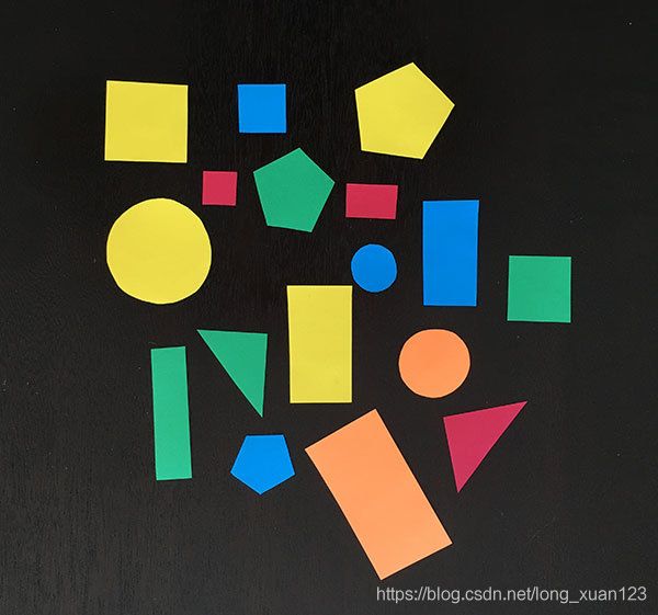
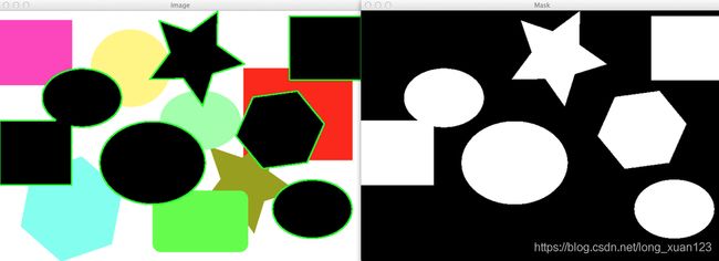
2. 查找图像中的形状

我们的目标:检测图像中的黑色形状。
使用cv2.inRange函数实际上很容易检测到这些黑色形状:
# import the necessary packages
import numpy as np
import argparse
import imutils
import cv2

# construct the argument parse and parse the arguments
ap = argparse.ArgumentParser()
ap.add_argument("-i", "--image", help = "path to the image file")
args = vars(ap.parse_args())

# load the image
image = cv2.imread(args["image"])

# find all the 'black' shapes in the image
lower = np.array([0, 0, 0])
upper = np.array([15, 15, 15])
shapeMask = cv2.inRange(image, lower, upper)

# find the contours in the mask
cnts = cv2.findContours(shapeMask.copy(), cv2.RETR_EXTERNAL,
	cv2.CHAIN_APPROX_SIMPLE)
cnts = imutils.grab_contours(cnts)
print("I found {} black shapes".format(len(cnts)))
cv2.imshow("Mask", shapeMask)

# loop over the contours
for c in cnts:
	# draw the contour and show it
	cv2.drawContours(image, [c], -1, (0, 255, 0), 2)
	cv2.imshow("Image", image)
	cv2.waitKey(0)
在第16和17行上,我们在BGR颜色空间中定义了上下边界点。 请记住,OpenCV以BGR顺序而不是RGB顺序存储图像。
我们的下边界由纯黑色组成,分别为蓝色,绿色和红色通道中的每个指定零。
我们的上限由一个非常深的灰色阴影组成,这次为每个通道指定15。
然后,我们在第18行的上下限范围内找到所有像素。
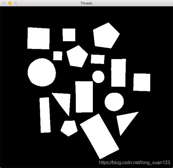
我们的shapeMask现在看起来像这样:
如您所见,原始图像中的所有黑色形状现在在黑色背景上均为白色。
下一步是检测shapeMask中的轮廓。 这也很简单:
我们在第21和22行调用cv2.findContours,指示它找到形状的所有外部轮廓(即边界)。
由于各种版本的OpenCV处理轮廓的方式不同,我们在第23行分析了轮廓。
从那里,我们将找到的轮廓数量打印到控制台。
然后,我们开始在第28行上循环遍历各个轮廓,并在第30行上将形状的轮廓绘制到原始图像上。
3. 查找轮廓中的极点
我将演示如何沿轮廓找到最北,南,东和西(x,y)坐标,就像本博文顶部的图像一样。
尽管这项技能本身并不是天生就有用的,但通常被用作更高级的计算机视觉应用程序的预处理步骤。 手势识别就是一个很好的例子。
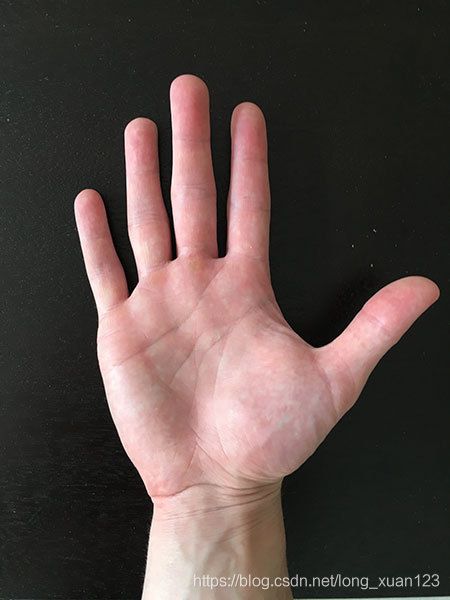
我们的目标是计算图像中手部轮廓的极限点。
# import the necessary packages
import imutils
import cv2

# load the image, convert it to grayscale, and blur it slightly
image = cv2.imread("hand_01.png")
gray = cv2.cvtColor(image, cv2.COLOR_BGR2GRAY)
gray = cv2.GaussianBlur(gray, (5, 5), 0)

# threshold the image, then perform a series of erosions +
# dilations to remove any small regions of noise
thresh = cv2.threshold(gray, 45, 255, cv2.THRESH_BINARY)[1]
thresh = cv2.erode(thresh, None, iterations=2)
thresh = cv2.dilate(thresh, None, iterations=2)

# find contours in thresholded image, then grab the largest
# one
cnts = cv2.findContours(thresh.copy(), cv2.RETR_EXTERNAL,
	cv2.CHAIN_APPROX_SIMPLE)
cnts = imutils.grab_contours(cnts)
c = max(cnts, key=cv2.contourArea)

# determine the most extreme points along the contour
extLeft = tuple(c[c[:, :, 0].argmin()][0])
extRight = tuple(c[c[:, :, 0].argmax()][0])
extTop = tuple(c[c[:, :, 1].argmin()][0])
extBot = tuple(c[c[:, :, 1].argmax()][0])

# draw the outline of the object, then draw each of the
# extreme points, where the left-most is red, right-most
# is green, top-most is blue, and bottom-most is teal
cv2.drawContours(image, [c], -1, (0, 255, 255), 2)
cv2.circle(image, extLeft, 8, (0, 0, 255), -1)
cv2.circle(image, extRight, 8, (0, 255, 0), -1)
cv2.circle(image, extTop, 8, (255, 0, 0), -1)
cv2.circle(image, extBot, 8, (255, 255, 0), -1)
# show the output image
cv2.imshow("Image", image)
cv2.waitKey(0)
第2行和第3行导入我们所需的包。 然后,我们从磁盘加载示例图像,将其转换为灰度,然后稍微高斯模糊。
第12行执行阈值处理,使我们能够将手部区域与其余图像分开。 阈值化后,我们的二进制图像如下所示:

为了检测手的轮廓,我们调用cv2.findContours,然后对轮廓进行排序以找到最大的轮廓,我们假定是手本身(第18-21行)。
在我们沿着轮廓找到极限点之前,重要的是要了解轮廓只是(x,y)坐标的NumPy数组。 因此,我们可以利用NumPy函数来帮助我们找到极限坐标。
例如,第24行通过调用x值上的argmin()并获取与x值关联的整个(x,y)坐标来找到整个轮廓数组c中最小的x坐标(即“西”值)。 argmin()返回的索引。
同样,第25行使用argmax()函数在轮廓数组中找到最大的x坐标(即“东”值)。
第26和27行仅对y坐标执行相同的操作,分别为我们提供“北”和“南”坐标。
现在我们有了极端的北,南,东和西坐标,我们可以在图像上绘制它们

4 轮廓排序
- 根据轮廓的大小/区域对轮廓进行排序,并按照模板按照其他任意标准对轮廓进行排序。
- 仅使用一个功能就可以从左到右,从右到左,从上到下以及从下到上对轮廓区域进行排序。
# import the necessary packages
import numpy as np
import argparse
import imutils
import cv2

def sort_contours(cnts, method="left-to-right"):
	# initialize the reverse flag and sort index
	reverse = False
	i = 0

	# handle if we need to sort in reverse
	if method == "right-to-left" or method == "bottom-to-top":
		reverse = True

	# handle if we are sorting against the y-coordinate rather than
	# the x-coordinate of the bounding box
	if method == "top-to-bottom" or method == "bottom-to-top":
		i = 1

	# construct the list of bounding boxes and sort them from top to
	# bottom
	boundingBoxes = [cv2.boundingRect(c) for c in cnts]
	(cnts, boundingBoxes) = zip(*sorted(zip(cnts, boundingBoxes),
		key=lambda b:b[1][i], reverse=reverse))

	# return the list of sorted contours and bounding boxes
	return (cnts, boundingBoxes)

def draw_contour(image, c, i):
	# compute the center of the contour area and draw a circle
	# representing the center
	M = cv2.moments(c)
	cX = int(M["m10"] / M["m00"])
	cY = int(M["m01"] / M["m00"])

	# draw the countour number on the image
	cv2.putText(image, "#{}".format(i + 1), (cX - 20, cY), cv2.FONT_HERSHEY_SIMPLEX,
		1.0, (255, 255, 255), 2)

	# return the image with the contour number drawn on it
	return image

# construct the argument parser and parse the arguments
ap = argparse.ArgumentParser()
ap.add_argument("-i", "--image", required=True, help="Path to the input image")
ap.add_argument("-m", "--method", required=True, help="Sorting method")
args = vars(ap.parse_args())

# load the image and initialize the accumulated edge image
image = cv2.imread(args["image"])
accumEdged = np.zeros(image.shape[:2], dtype="uint8")

# loop over the blue, green, and red channels, respectively
for chan in cv2.split(image):
	# blur the channel, extract edges from it, and accumulate the set
	# of edges for the image
	chan = cv2.medianBlur(chan, 11)
	edged = cv2.Canny(chan, 50, 200)
	accumEdged = cv2.bitwise_or(accumEdged, edged)

# show the accumulated edge map
cv2.imshow("Edge Map", accumEdged)

# find contours in the accumulated image, keeping only the largest
# ones
cnts = cv2.findContours(accumEdged.copy(), cv2.RETR_EXTERNAL,
	cv2.CHAIN_APPROX_SIMPLE)
cnts = imutils.grab_contours(cnts)
cnts = sorted(cnts, key=cv2.contourArea, reverse=True)[:5]
orig = image.copy()

# loop over the (unsorted) contours and draw them
for (i, c) in enumerate(cnts):
	orig = draw_contour(orig, c, i)

# show the original, unsorted contour image
cv2.imshow("Unsorted", orig)

# sort the contours according to the provided method
(cnts, boundingBoxes) = sort_contours(cnts, method=args["method"])

# loop over the (now sorted) contours and draw them
for (i, c) in enumerate(cnts):
	draw_contour(image, c, i)

# show the output image
cv2.imshow("Sorted", image)
cv2.waitKey(0)
我们将从导入必要的程序包开始:NumPy用于数值处理,argparse用于解析命令行参数,cv2用于我们的OpenCV绑定。
让我们暂时跳过这些步骤,然后立即跳入定义我们的sort_contours函数,该函数使我们能够对轮廓进行排序,而不必先解析参数,加载图像并执行其他常规过程,而不必从头开始。
实际的sort_contours函数在第7行中定义,并带有两个参数。第一个是cnts,我们要排序的轮廓列表,第二个是sorting方法,它指示我们要对轮廓进行排序的方向(即,从左到右,从上到下等)。
从那里,我们将在第9行和第10行上初始化两个重要的变量。这些变量仅表示排序顺序(升序或降序)以及我们将用于执行排序的边界框的索引(稍后会详细介绍)。我们将初始化这些变量,使其以升序排列,并沿着轮廓的边界框的x轴位置排列。
如果是从右到左或从下到上排序,则需要根据图像中轮廓的位置以降序排序(第13和14行)。
同样,在第18行和第19行,我们检查是从上到下还是从下到上进行排序。如果是这种情况,那么我们需要根据y轴值而不是x轴进行排序(因为我们现在是垂直而非水平排序)。
轮廓的实际排序发生在第23-25行。
我们首先计算每个轮廓的边界框,它只是边界框的起始(x,y)坐标,然后是宽度和高度(因此称为“边界框”)。 (第23行)
boundingBoxes使我们能够对实际的轮廓进行排序,我们使用一些Python魔术在第24行和第25行上对两个列表进行了排序。使用此代码,我们可以根据我们提供的标准对轮廓和边界框进行排序。
最后,我们将边界框和轮廓的(现在已排序)列表返回到第28行的调用函数。
在此过程中,让我们继续定义另一个帮助器函数draw_contour。
此函数仅在第33-35行上计算所提供轮廓c的中心(x,y)坐标,然后使用该中心坐标在第38和39行上绘制轮廓ID i。
最后,传入的图像返回到第42行的调用函数。
同样,这只是一个辅助功能,我们将利用它在实际图像上绘制轮廓ID号,以便可视化工作结果。
现在已经完成了辅助功能,让我们将驱动程序代码放置在适当的位置以拍摄实际图像,检测轮廓并对其进行排序。
第45-48行不是很有趣-它们只是解析我们的命令行参数,--image是我们的图像在磁盘上的驻留路径,而--method是我们想要的方向的文本表示。 整理轮廓。
从那里,我们将图像从第51行的磁盘上加载下来,并在第52行的边缘图上分配内存。
构造实际的边缘贴图发生在第55-60行,我们在图像的每个蓝色,绿色和红色通道(第55行)上循环,对每个通道略微模糊以消除高频噪声(第58行),执行边缘检测, (第59行),并在第60行上更新累积的边缘贴图。
我们在第63行显示累积的边缘图,如下所示:
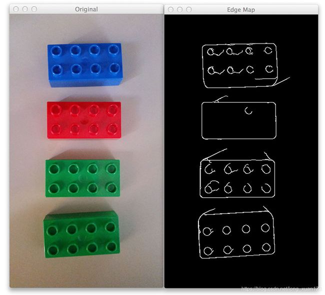
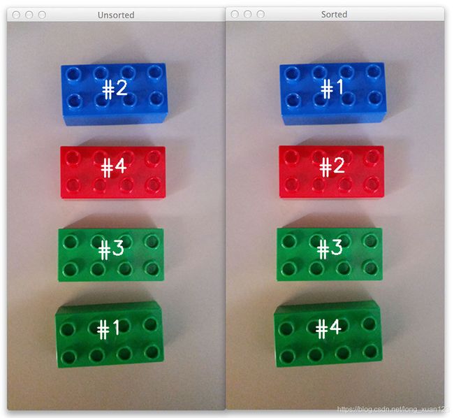
如您所见,我们已经检测到图像中乐高积木的实际边缘轮廓。
现在,让我们看看是否可以
(1)找到这些乐高积木的轮廓,
(2)然后对它们进行排序。
很显然,这里的第一步是在67-69行的累积边缘地图图像中找到实际轮廓。我们正在寻找乐高积木的外部轮廓,该轮廓仅与它们的轮廓相对应。
基于这些轮廓,我们现在将结合使用Python排序函数和cv2.contourArea方法根据它们的大小对它们进行排序-这使我们能够根据轮廓的面积(即大小)从最大到最大对它们进行排序。最小(第70行)。
我们采用这些排序的轮廓(就大小而言,而不是位置),在74行上对其进行循环,并使用draw_contour辅助函数在76行上绘制各个轮廓。
该图像然后显示在第78行的屏幕上。
但是,您会注意到,我们的轮廓仅根据其大小进行了排序-并未关注其在图像中的实际位置。
我们在第81行上解决了这个问题,我们在其中调用了自定义sort_contours函数。此方法接受我们的轮廓列表以及排序方向方法(通过命令行参数提供),并对它们进行排序,分别返回已排序的边界框和轮廓的元组。
最后,我们采用这些已排序的轮廓,在其上循环,绘制每个轮廓,最后将输出图像显示在屏幕上(第84-89行)。