再想 DiMP 的 Train&&Tracking

前言：如果没有看过论文，可以看一下我写的论文解读 DIMP，然后与这篇结合看

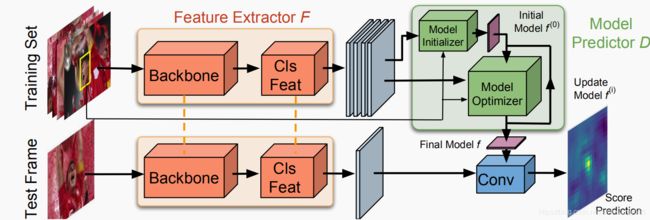
Training

Input

输入和ATOM不一样，它是五维tensor，（sequence ,batch,channel,width,height），上下两个分支分别输入的是3帧

Backbone

和ATOM一样，可以使用ResNet18也可以使用ResNet50，不一样的是，ATOM直接用预训练的参数，不fine-tine，而DiMP会优惠Backone的参数，具体代码如下：

 # Optimizer
    optimizer = optim.Adam([{'params': actor.net.classifier.filter_initializer.parameters(), 'lr': 5e-5},
                            {'params': actor.net.classifier.filter_optimizer.parameters(), 'lr': 5e-4},
                            {'params': actor.net.classifier.feature_extractor.parameters(), 'lr': 5e-5},
                            {'params': actor.net.bb_regressor.parameters(), 'lr': 1e-3},
                            {'params': actor.net.feature_extractor.parameters()}],
                           lr=2e-4)

这个就照应了文章强调的end-to-end train
The entire tracking network, including the target classification, bounding box estimation and
backbone modules, is trained offline on tracking datasets.

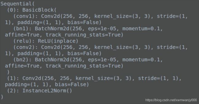
Clf Feat

在经过backbone提取特征之后，使用了特定的层将geneal feature 转换为 classified feature，那这个模块由什么构成的呢？如下：BasicBlock \ Conv2d \ InstanceL2Norm

The model predictor includes an initializer network that efficiently provides an initial estimate of the model weights, using only the target appearance. These weights are then processed by the optimizer module, taking both target and background samples into account.

于ATOM相比，它把在线的分类改为离线训练一个模型预测模块。

Model Predictor -----Model Initialization

初始化模块是由一个卷积层和一个PrPooling构成（用来在feature map 上提取bbox的特征），输入分类的特征（layer3）和bbox，得到初始的weights，经过PrPooling 后得到的pooled feature map 在所有的samples 平均得到最初的模型f

Model Predictor -----Model Optimaizer

输入得到的初始weights，bbox，分类层的特征，
We want to predict a target model f = D($S_{train}$)
那初始的weights怎么优化呢？ 就是本文提出的Discriminative Learning Loss：

第一项是残差项，第二项是正则化项
其中x * f计算的是score，c表示以目标中心的坐标c，一般我们使用：

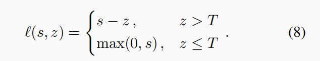
计算残差，$y_c$表示 Gaussian function centered at c，然而对于所有的负样本，需要强制模型学习到可靠的置信分，通常为0，这样模型只关注于负样本而不是获得判别能力，同时也不能解决正负样本不平衡的问题。因此他结合使用了least-squares 和 hinge loss，如下：

$m_c$表示target region，$v_c$表示spatial weight function
使用hinge loss的好处是，模型与曾背景中的容易样本，得到的大量负值，没有加在loss里面

确定loss后，使用什么优化器呢？如果使用梯度下降（GD），如下：

但是发现这个优化器需要大量的迭代，对参数f优化慢（The slow convergence of gradient descent is largely due
to the constant step length α, which does not depend on data or the current model estimate.）因此论文使用SD（seepest descent）去计算step length ,如下：

训练好Model Optimaizer后就可以应用到test 分支，优化结构如下：

Classification

使用如下loss进行分类层的优化：（也就是应用到test 分支，得出最后的score predictions）


where T = 0.05

分类的结构如下：

LinearFilter(
  (filter_initializer): FilterInitializerLinear(
    (filter_conv): Conv2d(256, 256, kernel_size=(3, 3), stride=(1, 1), padding=(1, 1))
    (filter_pool): FilterPool(
      (prroi_pool): PrRoIPool2D(kernel_size=(4, 4), spatial_scale=0.0625)
    )
  )
  (filter_optimizer): DiMPSteepestDescentGN(
    (distance_map): DistanceMap()
    (label_map_predictor): Conv2d(100, 1, kernel_size=(1, 1), stride=(1, 1), bias=False)
    (target_mask_predictor): Sequential(
      (0): Conv2d(100, 1, kernel_size=(1, 1), stride=(1, 1), bias=False)
      (1): Sigmoid()
    )
    (spatial_weight_predictor): Conv2d(100, 1, kernel_size=(1, 1), stride=(1, 1), bias=False)
    (score_activation): LeakyReluPar()
    (score_activation_deriv): LeakyReluParDeriv()
  )
  (feature_extractor): Sequential(
    (0): BasicBlock(
      (conv1): Conv2d(256, 256, kernel_size=(3, 3), stride=(1, 1), padding=(1, 1), bias=False)
      (bn1): BatchNorm2d(256, eps=1e-05, momentum=0.1, affine=True, track_running_stats=True)
      (relu): ReLU(inplace)
      (conv2): Conv2d(256, 256, kernel_size=(3, 3), stride=(1, 1), padding=(1, 1), bias=False)
      (bn2): BatchNorm2d(256, eps=1e-05, momentum=0.1, affine=True, track_running_stats=True)
    )
    (1): Conv2d(256, 256, kernel_size=(3, 3), stride=(1, 1), padding=(1, 1), bias=False)
    (2): InstanceL2Norm()
  )
)

Estimate target state

和ATOM一样
ATOM论文解读

ATOM代码运行一

ATOM代码运行二

ATOM代码运行三

Online Tracking

使用第一帧得到target model f，执行10次SD
.During tracking, we refine the target model f by performing two optimizer recursions every 20 frames, or a single recursion whenever a distractor peak is detected.
会建立一个memory来存储分类的特征，不超过50，使用这些特征来进行更新。

Training Details

比ATOM增加了GOT-10，使用四个数据集去训练
对于按照bbox 裁剪的时候，在原来target size的基础上扩大5倍
速度可以达到40FPS

Experiments

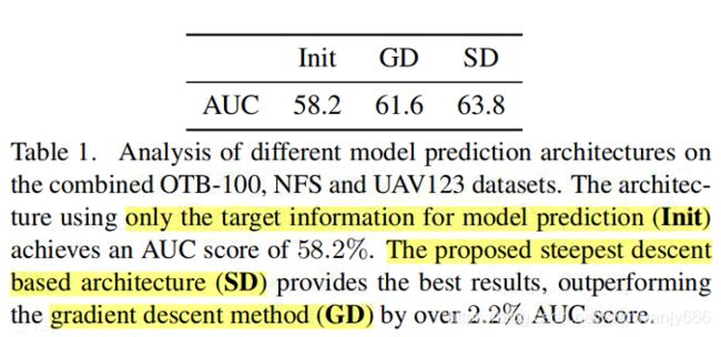
上面实验验证了优化模块的影响（Module Prediction），Init 表示仅仅使用初始模型来预测target model，移除了优化模块，这样就和Siamese方法一样，仅使用目标外观信息进行模型的预测，背景信息被丢弃。

上面这个验证了预测模块的影响。
The baseline SD constitutes our steepest descent based optimizer module along with the ImageNet pre-trained ResNet-18 network.That is, similar to the current state-of-the-art discriminative approaches, we do not fine-tune the backbone. I
+FT 表示训练 整个网络，包括backbone feature extractor
+Cls extract classification specific features

上面实验分析了在线更新的影响
OTB100 dimp50 0.684 dimp18 0.66
VOT2018 dimp50 0.440 dimp18 0.402
NFS dimp50 0.62 dimp18 0.61
UAV123 dimp50 0.654 dimp18 0.643
TrackingNet dimp50 0.74 dimp18 0.723
LaSoT dimp50 0.569 dimp18 0.535 （test 280 videos）
GOT-10k

补：与meta-learning 的不同

meta-learning framework employing an initial, target independent model, which is then refined using gradient descent with learned step-lengths. However, this strategy is only suitable for an initial adaption of the model and does not improve when applied in an iterative manner. This is due to the fact that it is not possible to learn constant step-lengths that accommodate both fast initial adaption and optimal convergence.

详细请看Meta-tracker

我想深度学习的魅力在于特征提取、loss设置和优化器的选择吧。