机器学习之线性回归python实现
-
- 一 理论基础
- 线性回归
- 岭回归
- lasso回归
- 局部加权线性回归
- 二 python实现
- 代码
- 结果
- 数据
- 一 理论基础
一. 理论基础
1. 线性回归
损失函数:
L(w)=12M∑i=1m(y−xiw)2
闭式解:
W=(XTX)−1XTY
如果 XTX 没有逆矩阵,则不能用这种方法,可以采用梯度下降等优化方法求近似解。
2. 岭回归
相当于在线性回归的基础上加了正则化。
损失函数:
L(w)=12m∑i=1m(y−xiw)2+λ∑i=1nw2i
闭式解:
W=(XTX+λI)−1XTY
3. lasso回归
相当于加了l1的正则化。
损失函数:
L(w)=12m∑i=1m(y−xiw)2+λ∑i=1n|wi|
这里不能采用闭式解,可以采用前向逐步回归。
4. 局部加权线性回归
给待测点附近的每个点赋予一定的权重。
损失函数:
L(θ)=12M∑i=1mwi(y−xiθ)2
其中, wi 表示第i个样本的权重。
局部加权线性回归使用”核“来对附近的点赋予更高的权重。核的类型可以自由选择,最常用的核就是高斯核,高斯核对应的权重如下:
wi=exp(|xi−x|−2k2)
这样就有一个只含对角元素的权重矩阵W, 并且点 xi 与x 越近, wi 也会越大。这里的参数k 决定了对附近的点赋予多大的权重,这也是唯一需要考虑的参数。
当k越大,有越多的点被用于训练回归模型;
当k越小,有越少的点用于训练回归模型。
二. python实现
1. 代码
#encoding=utf-8
###################################################################
#Copyright: CNIC
#Author: LiuYao
#Date: 2017-9-12
#Description: implements the linear regression algorithm
###################################################################

import numpy as np
from numpy.linalg import det
from numpy.linalg import inv
from numpy import mat
from numpy import random
import matplotlib.pyplot as plt
import pandas as pd

class LinearRegression:
    '''
    implements the linear regression algorithm class
    '''

    def __init__(self):
        pass

    def train(self, x_train, y_train):
        x_mat = mat(x_train).T
        y_mat = mat(y_train).T
        [m, n] = x_mat.shape
        x_mat = np.hstack((x_mat, mat(np.ones((m, 1)))))
        self.weight = mat(random.rand(n + 1, 1))
        if det(x_mat.T * x_mat) == 0:
            print 'the det of xTx is equal to zero.'
            return
        else:
            self.weight = inv(x_mat.T * x_mat) * x_mat.T * y_mat
        return self.weight

    def locally_weighted_linear_regression(self, test_point, x_train, y_train, k=1.0):
        x_mat = mat(x_train).T
        [m, n] = x_mat.shape
        x_mat = np.hstack((x_mat, mat(np.ones((m, 1)))))
        y_mat = mat(y_train).T
        test_point_mat = mat(test_point)
        test_point_mat = np.hstack((test_point_mat, mat([[1]])))
        self.weight = mat(np.zeros((n+1, 1)))
        weights = mat(np.eye((m)))
        test_data = np.tile(test_point_mat, [m,1])
        distances = (test_data - x_mat) * (test_data - x_mat).T / (n + 1)
        distances = np.exp(distances / (-2 * k ** 2))
        weights = np.diag(np.diag(distances))
        # weights = distances * weights
        xTx = x_mat.T * (weights * x_mat)
        if det(xTx) == 0.0:
            print 'the det of xTx is equal to zero.'
            return
        self.weight = xTx.I * x_mat.T * weights * y_mat
        return test_point_mat * self.weight

    def ridge_regression(self, x_train, y_train, lam=0.2):
        x_mat = mat(x_train).T
        [m, n] = np.shape(x_mat)
        x_mat = np.hstack((x_mat, mat(np.ones((m, 1)))))
        y_mat = mat(y_train).T
        self.weight = mat(random.rand(n + 1,1))
        xTx = x_mat.T * x_mat + lam * mat(np.eye(n))
        if det(xTx) == 0.0:
            print "the det of xTx is zero!"
            return
        self.weight = xTx.I * x_mat.T * y_mat
        return self.weight

    def lasso_regression(self, x_train, y_train, eps=0.01, itr_num=100):
        x_mat = mat(x_train).T
        [m,n] = np.shape(x_mat)
        x_mat = (x_mat - x_mat.mean(axis=0)) / x_mat.std(axis=0)
        x_mat = np.hstack((x_mat, mat(np.ones((m, 1)))))
        y_mat = mat(y_train).T
        y_mat = (y_mat - y_mat.mean(axis=0)) / y_mat.std(axis=0)
        self.weight = mat(random.rand(n+1, 1))
        best_weight = self.weight.copy()
        for i in range(itr_num):
            print self.weight.T
            lowest_error = np.inf
            for j in range(n + 1):
                for sign in [-1, 1]:
                    weight_copy = self.weight.copy()
                    weight_copy[j] += eps * sign
                    y_predict = x_mat * weight_copy
                    error = np.power(y_mat - y_predict, 2).sum()
                    if error < lowest_error:
                        lowest_error = error
                        best_weight = weight_copy
            self.weight = best_weight
        return self.weight

    def lwlr_predict(self, x_test, x_train, y_train, k=1.0):
        m = len(x_test)
        y_predict = mat(np.zeros((m, 1)))
        for i in range(m):
            y_predict[i] = self.locally_weighted_linear_regression(x_test[i], x_train, y_train, k)
        return y_predict


    def lr_predict(self, x_test):
        m = len(x_test)
        x_mat = np.hstack((mat(x_test).T, np.ones((m, 1))))
        return x_mat * self.weight

    def plot_lr(self, x_train, y_train):
        x_min = x_train.min()
        x_max = x_train.max()
        y_min = self.weight[0] * x_min + self.weight[1]
        y_max = self.weight[0] * x_max + self.weight[1]
        plt.scatter(x_train, y_train)
        plt.plot([x_min, x_max], [y_min[0,0], y_max[0,0]], '-g')
        plt.show()

    def plot_lwlr(self, x_train, y_train, k=1.0):
        x_min = x_train.min()
        x_max = x_train.max()
        x = np.linspace(x_min, x_max, 1000)
        y = self.lwlr_predict(x, x_train, y_train, k)
        plt.scatter(x_train, y_train)
        plt.plot(x, y.getA()[:, 0], '-g')
        plt.show()

    def plot_weight_with_lambda(self, x_train, y_train, lambdas):
        weights = np.zeros((len(lambdas), ))
        for i  in range(len(lambdas)):
            self.ridge_regression(x_train, y_train, lam=lambdas[i])
            weights[i] = self.weight[0]
        plt.plot(np.log(lambdas), weights)
        plt.show()

def main():
    data = pd.read_csv('/home/LiuYao/Documents/MarchineLearning/regression.csv')
    data = data / 30
    x_train = data['x'].values
    y_train = data['y'].values
    regression = LinearRegression()
    # regression.train(x_train, y_train)
    # y_predict = regression.predict(x_train)
    # regression.plot(x_train, y_train)
    # print '相关系数矩阵:', np.corrcoef(y_train, np.squeeze(y_predict))
    # y_predict = regression.lwlr_predict([[15],[20]], x_train, y_train, k=0.1)
    # print y_predict
    # regression.ridge_regression(x_train, y_train, lam=3)
    # regression.plot_lr(x_train, y_train)
    regression.lasso_regression(x_train, y_train, itr_num=1000)
    regression.plot_lr(x_train, y_train)

if __name__ == '__main__':
    main()
2. 结果


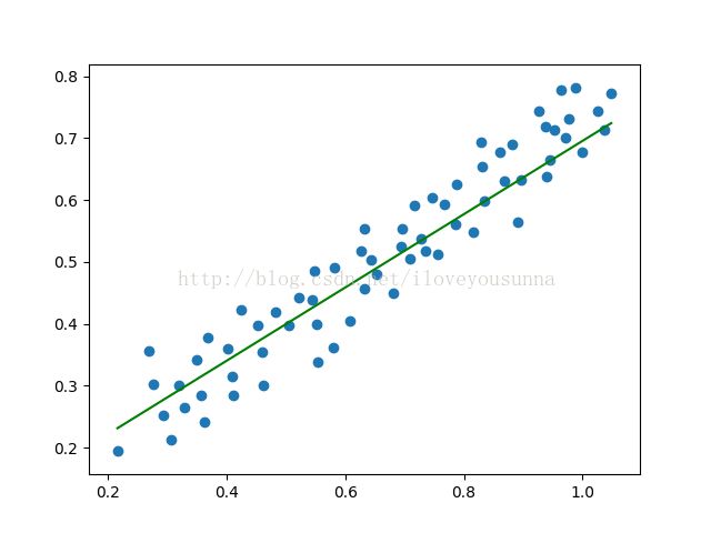

随着lambda的增大,意味着权值的惩罚越来越大,weight越来越小。

lasso回归倾向于将weight的某些维度压缩到0,比如例子中将weight的第二维压缩为0,使直线过原点;而岭回归倾向于使weight所有维度变小。
3. 数据
x,y
8.8,7.55
9.9,7.95
10.75,8.55
12.3,9.45
15.65,13.25
16.55,12.0
13.6,11.9
11.05,11.35
9.6,9.0
8.3,9.05
8.1,10.7
10.5,10.25
14.5,12.55
16.35,13.15
17.45,14.7
19.0,13.7
19.6,14.4
20.9,16.6
21.5,17.75
22.4,18.1
23.65,18.75
24.9,19.6
25.8,20.3
26.45,20.7
28.15,21.55
28.55,21.4
29.3,21.95
29.15,21.0
28.35,19.95
26.9,19.0
26.05,18.9
25.05,17.95
23.6,16.8
22.05,15.55
21.85,16.1
23.0,17.8
19.0,16.6
18.8,15.55
19.3,15.1
15.15,11.9
12.05,10.8
12.75,12.7
13.8,10.65
6.5,5.85
9.2,6.4
10.9,7.25
12.35,8.55
13.85,9.0
16.6,10.15
17.4,10.85
18.25,12.15
16.45,14.55
20.85,15.75
21.25,15.15
22.7,15.35
24.45,16.45
26.75,16.95
28.2,19.15
24.85,20.8
20.45,13.5
29.95,20.35
31.45,23.2
31.1,21.4
30.75,22.3
29.65,23.45
28.9,23.35
27.8,22.3