Consider a (two dimensional) data matrix with some values missing and you want to fill the holes by interpolated values. One particularly simple but at the same time powerful method is called Laplace interpolation.
The easy explanation goes as follows: for each missing value take the average over the 4 surrounding values, i.e. of the entries above, below, left and right. This holds for the inner points of the matrix, special rules apply to the borders, see below. Of course, maybe some or even all of the surrounding values are missing, too. In general this leads to a system of linear equations one has to solve.
The more involved explanation: search for a harmonic function interpolating the non-missing data. A harmonic function ![]() satisfies
satisfies
![]()
from which the mean value property follows. This says that each function value is the average of the function values on or in a surrounding sphere ![]()
![]()
where ![]() . That's deeper math of course. To find the harmonic function we have to solve its defining partial differential equation, which we discretize on the grid given by the data matrix itself assuming equidistant nodes (with distance say
. That's deeper math of course. To find the harmonic function we have to solve its defining partial differential equation, which we discretize on the grid given by the data matrix itself assuming equidistant nodes (with distance say ![]() ). For an inner point we have
). For an inner point we have
![]()
which is the same as
![]()
matching the easy explanation from the beginning. For each inner point of the matrix we either get this averaging equation, or if the data point is known to be ![]() simply
simply
![]()
This way we collect ![]() equations, if the original data matrix has
equations, if the original data matrix has ![]() rows and
rows and ![]() columns. The borders have modified equations, which I do not list here explicitly, but which are based on the conditions
columns. The borders have modified equations, which I do not list here explicitly, but which are based on the conditions ![]() for the upper and lower border,
for the upper and lower border, ![]() for the left and right border and
for the left and right border and ![]() for the four corners.
for the four corners.
Here is a tentative implementation in QuantLib using the BiCGStab solver at its heart.
Let’s do some examples (the code can be found here, together with a gnuplot scriptgenerating the pictures.
The original data is generated by filling a ![]() matrix
matrix sample like this
|
1
2
3
4
5
6
|
for
(Size i = 0; i < N; ++i) {
for
(Size j = 0; j < N; ++j) {
sample(i, j) =
sin
((
double
)(i + 1) / N * 4.0) *
cos
((
double
)(j + 1) / N * 4.0);
}
}
|
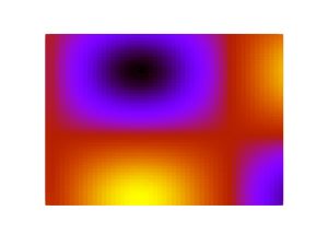
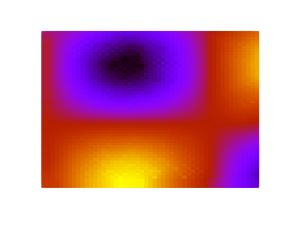
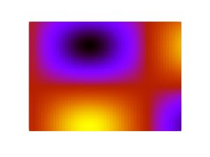
By the way, the function generating the test data is not harmonic. Plotted as a heatmap it looks like this:
![]()
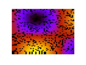
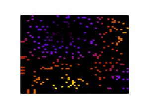
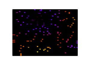
Now we delete ![]() of the points, randomly.
of the points, randomly.
We reconstruct the missing values by applying Laplace interpolation, which is done as easy as this
|
1
|
laplaceInterpolation(sample2);
|
where sample2 is the destructed matrix with missing values marked as Null. The function laplaceInterpolation replaces these values by interpolated ones and writes them back to the input matrix sample2.
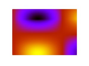
The reconstructed matrix looks is this:
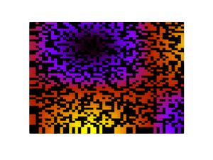
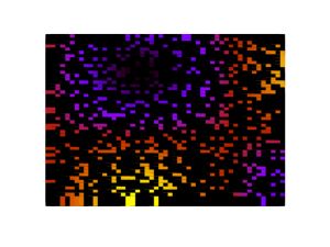
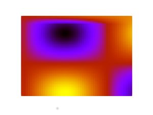
As beautiful as the original, isn’t it. Let’s delete more points and look and the reconstruction.
For ![]() we get
we get
for ![]() it is
it is
for ![]()
and for ![]()
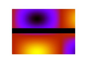
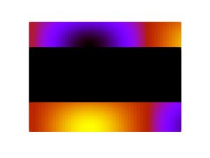
Quite amazing. Let’s look at how well the method works if we do not delete points randomly, but erase a whole stripe at the center of the matrix.
If the stripe is ![]() of the height
of the height
for ![]()
![]()
and for ![]()
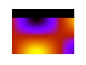
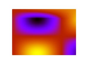
What about extrapolation? So let’s delete a stripe at the top of the matrix.
For ![]() we get
we get
for ![]()
and for ![]()
Of course the method can not see what is no longer there. Still it is working surprisingly well if you ask me.
quoted from: https://quantlib.wordpress.com/2015/11/21/laplace-interpolation/
