Spatial Transformer Networks
TF code: https://github.com/kevinzakka/spatial-transformer-network
一、相关背景
如果网络能够对经过平移、旋转、缩放及裁剪等操作的图片得到与未经变换前相同的检测结果,我们就说这个网络具有空间变换不变性(将平移、旋转、缩放及裁剪不变性统称为空间不变性)。具有空间变换不变性的网络能够得到更精确地分类结果。传统CNN网络的池化层具有平移不变性(网络在平移小于池化矩阵的范围时具有平移不变性。所以只有平移小于这个范围,才能保证平移不变性。),但是CNN网络对于大尺度的空间变换并不具备不变性。Spatial Transformer Networks提出的空间网络变换层,具有平移不变性、旋转不变性及缩放不变性等强大的性能。这个网络可以加在现有的卷积网络中,提高分类的准确性。
如下图所示:输入手写字体,我们感兴趣的是黄色框中的包含数字的区域,那么在训练的过程中,学习到的空间变换网络会自动提取黄色框中的局部数据特征,并对框内的数据进行空间变换,得到输出output。综上所述,空间变换网络主要有如下三个作用:
- 可以将输入转换为下一层期望的形式
- 可以在训练的过程中自动选择感兴趣的区域特征
- 可以实现对各种形变的数据进行空间变换

图1.空间变换网络作用示意图
二、相关理论
在理解STN之前,先简单了解一下基本的仿射变换、双线性插值。
- 仿射变换(Affine transformation)
下面的所有变换假设都是针对一幅图像,即一个三维数组(H*W*C),这里为简单起见,假设图像都是单通道(C=1)的。首先说明一下待会要用到的符号:
- (x,y): 原图像中某一点A的位置
- (x′,y′): 变换后图像中A点对应的位置
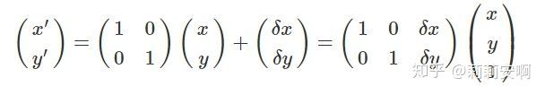
平移(translation)
若将原图像沿x和y方向分别平移 和 ,即:
写成矩阵形式如下:
缩放(Scaling)
假设将图像分别沿x和y方向分别缩放p倍和q倍,且p>0,q>0,即:
写成矩阵形式如下:

旋转(Rotation)

图2.旋转变换示意图
如上图所示,点A旋转θ角到点B,由B点可得
由A点可得:
整理可得
写成矩阵形式如下:

剪切(Shear)
剪切变换指的是类似于四边形不稳定性那种性质,方形变平行四边形。任意一边都可以被拉长,以一定比例的x补偿y,也以一定比例的y补偿x。

仿射变换(Affine transformation)
其实上面几种常见变换都可以用同一种变换来表示,就是仿射变换,它有更一般的形式,如下:
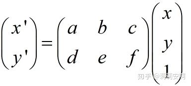
a,b,c,d,e,f取不同的值就可以表示上述不同的变换。当6个参数取其上述变换以外的值时,为一般的仿射变换,效果相当于从不同的位置看同一个目标。
2.双线性插值(Bilinear Interpolation)
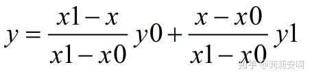
在对图像进行仿射变换时,会出现一个问题,当原图像中某一点的坐标映射到变换后图像时,坐标可能会出现小数,而我们知道,图像上某一像素点的位置坐标只能是整数,那该怎么办?这时候双线性插值就起作用了。在介绍双线性插值之前,先讲一下线性插值的计算方法:已知点 (x0, y0) 与 (x1, y1),要计算 [x0, x1] 区间内某一位置 x 在直线上的y值,可以采用两点式写出直线方程并求得y的取值如下:
双线性插值的基本思想是通过某一点周围四个点的灰度值来估计出该点的灰度值,如图3所示.
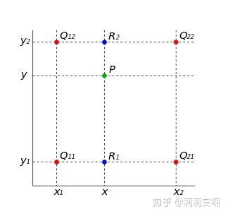
图3.双线性插值示意图
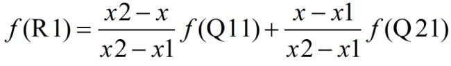
已知Q11、Q12、Q21、Q22四点的坐标,要求点P的坐标。分成两步,首先在 x 方向进行线性插值,得到:

然后在 y 方向进行线性插值,得到:
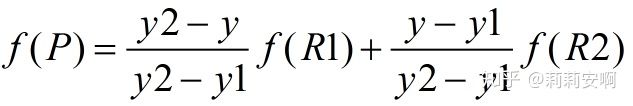
由于图像双线性插值只会用相邻的4个点,因此上述公式的分母都是1。整合上述公式有:
![]()
三、算法概述

STN网络包括三部分:
- Localisation Network-局部网络
- Parameterised Sampling Grid-参数化网格采样
- Differentiable Image Sampling-差分图像采样
- Localisation Network-局部网络
输入:特征图
输出:变换矩阵 ,用于下一步计算( 输出规模视具体的变换。以仿射变换为例, 是一个[2,3]大小的6维参数)
注: 被初始化为恒等变换矩阵,通过损失函数不断更正的参数,最终得到期望的仿射变换矩阵。得到输出特征图后最重要的是得到输出特征图每个位置的像素值。(图像对于计算机来说就是一个0-255的像素值组成的矩阵,图像经过空间变换后每个点的像素值肯定会发生变化,下面就介绍如何确定变换后的特征图每个位置的像素值)
2. Parameterised Sampling Grid-参数化网格采样
此步骤的目地是为了得到输出特征图的坐标点对应的输入特征图的坐标点的位置。计算方式如下:


式中s代表输入特征图像坐标点,t代表输出特征图坐标点, 是局部网络的输出。这里需要注意的是坐标的映射关系是从目标图片——>输入图片。这是因为输入图片与目标图片坐标点均是人为定义的标准化格点矩阵,x,y的值在-1到1之间,图片任何一个位置的坐标点是固定不变的。这就好比两个坐标完全一样的图像,无论用谁乘以仿射变换矩阵,都可以得到经过仿射变换后的图像与原坐标点的映射关系。也就是说这里即使把坐标的映射关系变为输入图片——>目标图片得到的也是一样的映射关系。至于为什么要使用前者来求解这种映射关系,个人理解的是目标图片是我们期望的输出,我们通常以输出为参考,依次获得目标图片在每个坐标点的像素值。比如目标图片坐标点(0,0)对应输入图片坐标点(3,1),我们就先取出输入图片坐标点(3,1)处的像素值,这样依次获得目标图片在每个坐标点的像素值。通过上面的解释相信你们也能理解为什么没有使用仿射变换的逆矩阵。
通过这一步,我们已经得到变换后的输出特征图每个位置的坐标在输入特征图上的对应坐标点。下面我们就可以直接提取出输入特征图的每个位置的像素值(tensorflow有专门的函数可以得到指定位置的像素值)。在提取像素值之前,我们应该注意到一点:目标图片的坐标点对应的输入图片的坐标点不一定是整数坐标点(例如目标图片坐标点(0,1)对应输入图片坐标点(3.2,1.3)),而仅仅整数坐标才能提取像素值,所以需要利用插值的方式来计算出对应该点的灰度值(像素值)。可以看出,步骤一为步骤二提供了仿射变换的矩阵,步骤二为步骤三提供了输出特征图的坐标点对应的输入特征图的坐标点的位置,步骤三只需要提取这个对应的坐标点的像素值(非整数坐标需要使用双向性插值提取像素值)就能最终得到输出特征图V。

左图为输出特征图 右图为输入特征图
3.Differentiable Image Sampling-差分图像采样
这一步完成的任务就是利用期望的插值方式来计算出对应点的灰度值。这里以双向性插值为例讲解,论文中给出了双向性插值的计算公式如下:
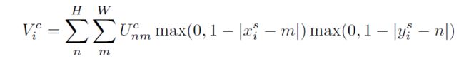
为输出特征图上第c个通道某一点的灰度值, 为输入特征图上第c个通道点(n,m)的灰度。当或者大于1时,对应的max()项将取0,也就是说,只有 周围4个点的灰度值决定目标像素点的灰度。并且当 和 越小,影响越大(即离点 (n,m)越近),权重越大,这和我们上面介绍双线性插值的结论是一致的。其实,这个式子等价于下式:
![]()
四、总结及代码实现-代码下载
1.Spatial Transformer Networks代码实现
def transformer(U, theta, out_size, name='SpatialTransformer', **kwargs):
	print('begin-transformer')

	def _repeat(x, n_repeats):
		with tf.variable_scope('_repeat'):
			rep = tf.transpose(
				tf.expand_dims(tf.ones(shape=tf.stack([n_repeats, ])), 1), [1, 0])
			rep = tf.cast(rep, 'int32')
			x = tf.matmul(tf.reshape(x, (-1, 1)), rep)
			return tf.reshape(x, [-1])

	def _interpolate(im, x, y, out_size):
		with tf.variable_scope('_interpolate'):
			# constants
			num_batch = tf.shape(im)[0]
			height = tf.shape(im)[1]
			width = tf.shape(im)[2]
			channels = tf.shape(im)[3]

			x = tf.cast(x, 'float32')
			y = tf.cast(y, 'float32')
			height_f = tf.cast(height, 'float32')
			width_f = tf.cast(width, 'float32')
			out_height = out_size[0]
			out_width = out_size[1]
			zero = tf.zeros([], dtype='int32')
			max_y = tf.cast(tf.shape(im)[1] - 1, 'int32')
			max_x = tf.cast(tf.shape(im)[2] - 1, 'int32')

			# scale indices from [-1, 1] to [0, width/height]
			x = (x + 1.0) * (width_f) / 2.0
			y = (y + 1.0) * (height_f) / 2.0

			# do sampling
			x0 = tf.cast(tf.floor(x), 'int32')
			x1 = x0 + 1
			y0 = tf.cast(tf.floor(y), 'int32')
			y1 = y0 + 1

			x0 = tf.clip_by_value(x0, zero, max_x)
			x1 = tf.clip_by_value(x1, zero, max_x)
			y0 = tf.clip_by_value(y0, zero, max_y)
			y1 = tf.clip_by_value(y1, zero, max_y)
			dim2 = width
			dim1 = width * height
			base = _repeat(tf.range(num_batch) * dim1, out_height * out_width)
			base_y0 = base + y0 * dim2
			base_y1 = base + y1 * dim2
			idx_a = base_y0 + x0
			idx_b = base_y1 + x0
			idx_c = base_y0 + x1
			idx_d = base_y1 + x1

			# use indices to lookup pixels in the flat image and restore
			# channels dim
			im_flat = tf.reshape(im, tf.stack([-1, channels]))
			im_flat = tf.cast(im_flat, 'float32')
			Ia = tf.gather(im_flat, idx_a)
			Ib = tf.gather(im_flat, idx_b)
			Ic = tf.gather(im_flat, idx_c)
			Id = tf.gather(im_flat, idx_d)

			# and finally calculate interpolated values
			x0_f = tf.cast(x0, 'float32')
			x1_f = tf.cast(x1, 'float32')
			y0_f = tf.cast(y0, 'float32')
			y1_f = tf.cast(y1, 'float32')
			wa = tf.expand_dims(((x1_f - x) * (y1_f - y)), 1)
			wb = tf.expand_dims(((x1_f - x) * (y - y0_f)), 1)
			wc = tf.expand_dims(((x - x0_f) * (y1_f - y)), 1)
			wd = tf.expand_dims(((x - x0_f) * (y - y0_f)), 1)
			output = tf.add_n([wa * Ia, wb * Ib, wc * Ic, wd * Id])
			return output

	def _meshgrid(height, width):
		print('begin--meshgrid')
		with tf.variable_scope('_meshgrid'):
			# This should be equivalent to:
			#  x_t, y_t = np.meshgrid(np.linspace(-1, 1, width),
			#                         np.linspace(-1, 1, height))
			#  ones = np.ones(np.prod(x_t.shape))
			#  grid = np.vstack([x_t.flatten(), y_t.flatten(), ones])

			x_t = tf.matmul(tf.ones(shape=tf.stack([height, 1])),
			                tf.transpose(tf.expand_dims(tf.linspace(-1.0, 1.0, width), 1), [1, 0]))
			print('meshgrid_x_t_ok')
			y_t = tf.matmul(tf.expand_dims(tf.linspace(-1.0, 1.0, height), 1),
			                tf.ones(shape=tf.stack([1, width])))
			print('meshgrid_y_t_ok')
			x_t_flat = tf.reshape(x_t, (1, -1))
			y_t_flat = tf.reshape(y_t, (1, -1))
			print('meshgrid_flat_t_ok')
			ones = tf.ones_like(x_t_flat)
			print('meshgrid_ones_ok')
			print(x_t_flat)
			print(y_t_flat)
			print(ones)

			grid = tf.concat([x_t_flat, y_t_flat, ones], 0)
			print('over_meshgrid')
			return grid

	def _transform(theta, input_dim, out_size):
		print('_transform')

		with tf.variable_scope('_transform'):
			num_batch = tf.shape(input_dim)[0]
			height = tf.shape(input_dim)[1]
			width = tf.shape(input_dim)[2]
			num_channels = tf.shape(input_dim)[3]
			theta = tf.reshape(theta, (-1, 2, 3))
			theta = tf.cast(theta, 'float32')

			# grid of (x_t, y_t, 1), eq (1) in ref [1]
			height_f = tf.cast(height, 'float32')
			width_f = tf.cast(width, 'float32')
			out_height = out_size[0]
			out_width = out_size[1]
			grid = _meshgrid(out_height, out_width)
			grid = tf.expand_dims(grid, 0)
			grid = tf.reshape(grid, [-1])
			grid = tf.tile(grid, tf.stack([num_batch]))
			grid = tf.reshape(grid, tf.stack([num_batch, 3, -1]))
			# tf.batch_matrix_diag
			# Transform A x (x_t, y_t, 1)^T -> (x_s, y_s)
			print('begin--batch--matmul')
			T_g = tf.matmul(theta, grid)
			x_s = tf.slice(T_g, [0, 0, 0], [-1, 1, -1])
			y_s = tf.slice(T_g, [0, 1, 0], [-1, 1, -1])
			x_s_flat = tf.reshape(x_s, [-1])
			y_s_flat = tf.reshape(y_s, [-1])

			input_transformed = _interpolate(
				input_dim, x_s_flat, y_s_flat,
				out_size)

			output = tf.reshape(
				input_transformed, tf.stack([num_batch, out_height, out_width, num_channels]))
			print('over_transformer')
			return output

	with tf.variable_scope(name):
		output = _transform(theta, U, out_size)
		return output


def batch_transformer(U, thetas, out_size, name='BatchSpatialTransformer'):
	with tf.variable_scope(name):
		num_batch, num_transforms = map(int, thetas.get_shape().as_list()[:2])
		indices = [[i] * num_transforms for i in xrange(num_batch)]
		input_repeated = tf.gather(U, tf.reshape(indices, [-1]))
		return transformer(input_repeated, thetas, out_size)
2.STN网络测试代码
from scipy import ndimage
import tensorflow as tf
from STN_tf_01 import transformer
import numpy as np
import matplotlib.pyplot as plt
import cv2

im = ndimage.imread('C:\\Users\julie\Desktop\cat.jpg')#改为你自己要测试的图片路径
im = im / 255.
# im=tf.reshape(im, [1,1200,1600,3])

im = im.reshape(1, 1200, 1600, 3)

im = im.astype('float32')
print('img-over')
out_size = (600, 800)
batch = np.append(im, im, axis=0)
batch = np.append(batch, im, axis=0)
num_batch = 3

x = tf.placeholder(tf.float32, [None, 1200, 1600, 3])
x = tf.cast(batch, 'float32')
print('begin---')
with tf.variable_scope('spatial_transformer_0'):
	n_fc = 6
	w_fc1 = tf.Variable(tf.Variable(tf.zeros([1200 * 1600 * 3, n_fc]), name='W_fc1'))
	initial = np.array([[0.5, 0, 0], [0, 0.5, 0]])
	initial = initial.astype('float32')
	initial = initial.flatten()

	b_fc1 = tf.Variable(initial_value=initial, name='b_fc1')

	h_fc1 = tf.matmul(tf.zeros([num_batch, 1200 * 1600 * 3]), w_fc1) + b_fc1

	print(x, h_fc1, out_size)

	h_trans = transformer(x, h_fc1, out_size)

sess = tf.Session()
sess.run(tf.global_variables_initializer())
y = sess.run(h_trans, feed_dict={x: batch})
plt.imshow(y[0])
plt.show()
   效果如下:
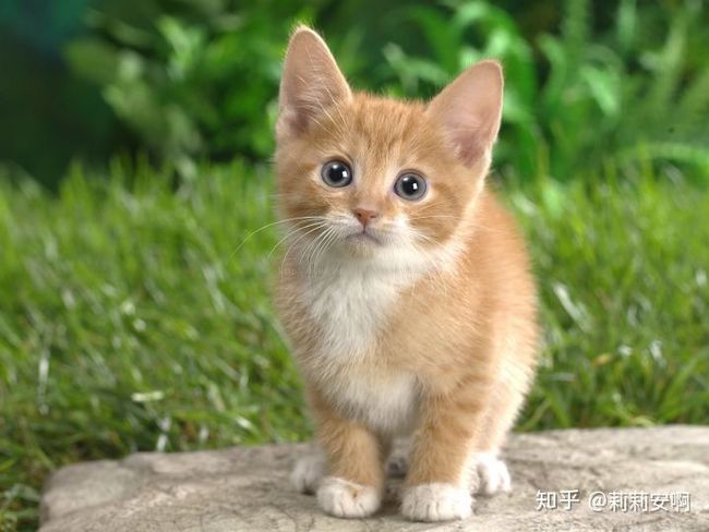
输入图片
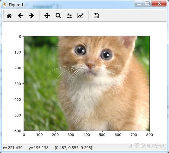
经过STN网络的图片