2020-8-1 吴恩达-改善深层NN-w1 深度学习的实用层面(课后编程3-Gradient Checking)
原文链接
如果打不开,也可以复制链接到https://nbviewer.jupyter.org中打开。
梯度检验 Gradient Checking
- 1.梯度检验如何工作
- 2.一维梯度检验
- 2-1.前向传播
- 2-2.反向传播
- 2-3.梯度检验
- 3.N维梯度检验
- 3-1.前向传播
- 3-2.反向传播
- 3-3.梯度检查
- 4.全代码
欢迎来到本周最后一个作业。通过本作业你将学习如何实现和使用梯度检验。
你是一个团队的一员,致力于全球范围的移动支付系统。你被要求建立一个DL模型来检测欺诈行为——每当有人进行支付时,你都要看看支付是否有欺诈行为,比如用户的账户是否被黑。
但是反向传播的实现非常有调整性,有时还存在缺陷。因为这是一个关键任务系统,所以你公司的CEO希望确定你反向传播的实现是正确的。你的CEO说:“给我证据证明你的反向传播是有效的”。为了确保这一点,你需要使用“梯度检验”。
加载库
# Packages
import numpy as np
from testCases import *
from gc_utils import sigmoid, relu, dictionary_to_vector, vector_to_dictionary, gradients_to_vector
1.梯度检验如何工作
反向传播计算梯度 ∂ J ∂ θ \frac{\partial J}{\partial \theta} ∂θ∂J, θ \theta θ 表示模型中的参数。使用前向传播和你的损失函数来计算 J J J 。
因为前向传播相对容易实现,你有信心你是正确的,所以你100%确信你的成本 J J J的计算是正确的。因此,你可以使用你计算 J J J的代码来验证计算 ∂ J ∂ θ \frac{\partial J}{\partial \theta} ∂θ∂J的代码。
让我们来回顾一下导数(或者说梯度)的定义。
∂ J ∂ θ = lim ε → 0 J ( θ + ε ) − J ( θ − ε ) 2 ε (1) \frac{\partial J}{\partial \theta} = \lim_{\varepsilon \to 0} \frac{J(\theta + \varepsilon) - J(\theta - \varepsilon)}{2 \varepsilon} \tag{1} ∂θ∂J=ε→0lim2εJ(θ+ε)−J(θ−ε)(1)
- ∂ J ∂ θ \frac{\partial J}{\partial \theta} ∂θ∂J是你想确保你计算正确的值。
- 因为你确信成本 J J J的实现是正确的,所以你能够计算 J ( θ + ε ) J(\theta + \varepsilon) J(θ+ε)和 J ( θ − ε ) J(\theta - \varepsilon) J(θ−ε) ( θ \theta θ是一个实数)。
现在你可以使用公式(1)和一个小的值的 ε \varepsilon ε来说服你的CEO,你计算 ∂ J ∂ θ \frac{\partial J}{\partial \theta} ∂θ∂J 的代码是正确的。
2.一维梯度检验
考虑一维线性方程 J ( θ ) = θ x J(\theta) = \theta x J(θ)=θx。这个模型只有一个实数值参数 θ \theta θ, x x x 是输入。
你将实现计算 J ( . ) J(.) J(.)和它的导数 ∂ J ∂ θ \frac{\partial J}{\partial \theta} ∂θ∂J的代码。然后你用梯度检验来确保关于 J J J的导数计算是正确的。

上图展示了关键计算步骤:从输入 x x x 开始,然后计算函数 J ( x ) J(x) J(x)(前向传播),最后计算 ∂ J ∂ θ \frac{\partial J}{\partial \theta} ∂θ∂J (反向传播)。
练习:为了这个简单的函数实现前向传播和反向传播。即,计算 J ( . ) J(.) J(.)(前向传播)和它对 θ \theta θ 的导数(反向传播),前向传播和反向传播分别在2个单独的函数中实现。
2-1.前向传播
# GRADED FUNCTION: forward_propagation

def forward_propagation(x, theta):
    """
    Implement the linear forward propagation (compute J) presented in Figure 1 (J(theta) = theta * x)
    实现图中的线性前向传播(计算J)(J(theta)= theta * x)

    Arguments:
    x -- a real-valued input 实数值输入
    theta -- our parameter, a real number as well 参数,也是一个实数

    Returns:
    J -- the value of function J, computed using the formula J(theta) = theta * x
    函数J的值,用公式J(theta)= theta * x计算
    """

    ### START CODE HERE ### (approx. 1 line)
    J = np.dot(theta, x)
    ### END CODE HERE ###

    return J
测试一下
x, theta = 2, 4
J = forward_propagation(x, theta)
print ("J = " + str(J))
运行结果
J = 8
2-2.反向传播
练习:现在来实现上图中反向传播(导数计算)。它就是计算函数 J ( θ ) = θ x J(\theta) = \theta x J(θ)=θx 对 θ \theta θ的导数。为了节省微积分计算,你将得到 d t h e t a = ∂ J ∂ θ = x dtheta = \frac { \partial J }{ \partial \theta} = x dtheta=∂θ∂J=x。
# GRADED FUNCTION: backward_propagation

def backward_propagation(x, theta):
    """
    Computes the derivative of J with respect to theta (see Figure 1).
    计算J相对于θ的导数。

    Arguments:
    x -- a real-valued input
    theta -- our parameter, a real number as well

    Returns:
    dtheta -- the gradient of the cost with respect to theta
    成本J对于θ的梯度
    """

    ### START CODE HERE ### (approx. 1 line)
    dtheta = x
    ### END CODE HERE ###

    return dtheta
测试一下
x, theta = 2, 4
dtheta = backward_propagation(x, theta)
print ("dtheta = " + str(dtheta))
结果
dtheta = 2
2-3.梯度检验
指导:
- 首先使用公式(1)和小值的 ε \varepsilon ε计算gradapprox–近似梯度,步骤如下
- 1、 θ + = θ + ε \theta^{+} = \theta + \varepsilon θ+=θ+ε
- 2、 θ − = θ − ε \theta^{-} = \theta - \varepsilon θ−=θ−ε
- 3、 J + = J ( θ + ) J^{+} = J(\theta^{+}) J+=J(θ+)
- 4、 J − = J ( θ − ) J^{-} = J(\theta^{-}) J−=J(θ−)
- 5、 g r a d a p p r o x = J + − J − 2 ε gradapprox = \frac{J^{+} - J^{-}}{2 \varepsilon} gradapprox=2εJ+−J−
- 然后使用反向传播计算梯度,结果保存在变量grad
- 最后计算gradapprox和grad的差,公式如下 d i f f e r e n c e = ∣ ∣ g r a d − g r a d a p p r o x ∣ ∣ 2 ∣ ∣ g r a d ∣ ∣ 2 + ∣ ∣ g r a d a p p r o x ∣ ∣ 2 (2) difference = \frac {\mid\mid grad - gradapprox \mid\mid_2}{\mid\mid grad \mid\mid_2 + \mid\mid gradapprox \mid\mid_2} \tag{2} difference=∣∣grad∣∣2+∣∣gradapprox∣∣2∣∣grad−gradapprox∣∣2(2) 你将用三步来计算:
- 1、使用
np.linalg.norm(...)计算分子 - 2、使用
np.linalg.norm(...)2次,计算分母 - 3、两者相除
- 1、使用
- 如果差很小(比如小于 1 0 − 7 10^{-7} 10−7),你可以确信你的梯度计算是正确的。否则,梯度计算过程可能有错误。
# GRADED FUNCTION: gradient_check

def gradient_check(x, theta, epsilon=1e-7):
    """
    Implement the backward propagation presented in Figure 1.
    实现图中的反向传播。

    Arguments:
    x -- a real-valued input
    theta -- our parameter, a real number as well
    epsilon -- tiny shift to the input to compute approximated gradient with formula(1)
   使用公式(1)计算输入的微小偏移以计算近似梯度

    Returns:
    近似梯度和后向传播梯度之间的差异
    difference -- difference (2) between the approximated gradient and the backward propagation gradient
    """

    # Compute gradapprox using left side of formula (1). epsilon is small enough, you don't need to worry about the limit.
    ### START CODE HERE ### (approx. 5 lines)
    thetaplus = theta + epsilon                               # Step 1
    thetaminus = theta - epsilon                              # Step 2
    J_plus = forward_propagation(x, thetaplus)                # Step 3
    J_minus = forward_propagation(x, thetaminus)              # Step 4
    gradapprox = (J_plus - J_minus) / (2 * epsilon)           # Step 5
    ### END CODE HERE ###

    # Check if gradapprox is close enough to the output of backward_propagation()
    ### START CODE HERE ### (approx. 1 line)
    grad = backward_propagation(x, theta)
    ### END CODE HERE ###

    ### START CODE HERE ### (approx. 1 line)
    numerator = np.linalg.norm(grad - gradapprox)                      # Step 1'
    denominator = np.linalg.norm(grad) + np.linalg.norm(gradapprox)    # Step 2'
    difference = numerator / denominator                               # Step 3'
    ### END CODE HERE ###

    if difference < 1e-7:
        print("The gradient is correct!")
    else:
        print("The gradient is wrong!")

    return difference
测试一下
x, theta = 2, 4
difference = gradient_check(x, theta)
print("difference = " + str(difference))
结果
The gradient is correct!
difference = 2.919335883291695e-10
恭喜,差异小于 1 0 − 7 10^{-7} 10−7阈值。所以你可以确信你的反向传播backward_propagation()计算的梯度是正确的。
现在,更加一般的情况,你的成本函数 J J J 有不止一个输入。当你训练NN, θ \theta θ实际上有多个权重矩阵 W [ l ] W^{[l]} W[l] 和偏置 b [ l ] b^{[l]} b[l]组成。高维度输入如何进行梯度检验非常重要。
3.N维梯度检验
下图展示了你的欺诈检测模型前向传播和反向传播。
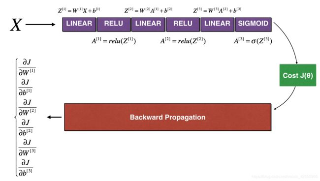
我们来看一下你的前向传播和反向传播的实现。
3-1.前向传播
def forward_propagation_n(X, Y, parameters):
    """
    Implements the forward propagation (and computes the cost) presented in Figure 3.

    Arguments:
    X -- training set for m examples
    Y -- labels for m examples
    parameters -- python dictionary containing your parameters "W1", "b1", "W2", "b2", "W3", "b3":
                    W1 -- weight matrix of shape (5, 4)
                    b1 -- bias vector of shape (5, 1)
                    W2 -- weight matrix of shape (3, 5)
                    b2 -- bias vector of shape (3, 1)
                    W3 -- weight matrix of shape (1, 3)
                    b3 -- bias vector of shape (1, 1)

    Returns:
    cost -- the cost function (logistic cost for one example)
    """

    # retrieve parameters
    m = X.shape[1]
    W1 = parameters["W1"]
    b1 = parameters["b1"]
    W2 = parameters["W2"]
    b2 = parameters["b2"]
    W3 = parameters["W3"]
    b3 = parameters["b3"]

    # LINEAR -> RELU -> LINEAR -> RELU -> LINEAR -> SIGMOID
    Z1 = np.dot(W1, X) + b1
    A1 = relu(Z1)
    Z2 = np.dot(W2, A1) + b2
    A2 = relu(Z2)
    Z3 = np.dot(W3, A2) + b3
    A3 = sigmoid(Z3)

    # Cost
    logprobs = np.multiply(-np.log(A3), Y) + np.multiply(-np.log(1 - A3), 1 - Y)
    cost = 1. / m * np.sum(logprobs)

    cache = (Z1, A1, W1, b1, Z2, A2, W2, b2, Z3, A3, W3, b3)

    return cost, cache
3-2.反向传播
def backward_propagation_n(X, Y, cache):
    """
    Implement the backward propagation presented in figure 2.

    Arguments:
    X -- input datapoint, of shape (input size, 1)
    Y -- true "label"
    cache -- cache output from forward_propagation_n()

    Returns:
    gradients -- A dictionary with the gradients of the cost with respect to each parameter, activation and pre-activation variables.
    """

    m = X.shape[1]
    (Z1, A1, W1, b1, Z2, A2, W2, b2, Z3, A3, W3, b3) = cache

    dZ3 = A3 - Y
    dW3 = 1. / m * np.dot(dZ3, A2.T)
    db3 = 1. / m * np.sum(dZ3, axis=1, keepdims=True)

    dA2 = np.dot(W3.T, dZ3)
    dZ2 = np.multiply(dA2, np.int64(A2 > 0))
    dW2 = 1. / m * np.dot(dZ2, A1.T) * 2  # Should not multiply by 2
    db2 = 1. / m * np.sum(dZ2, axis=1, keepdims=True)

    dA1 = np.dot(W2.T, dZ2)
    dZ1 = np.multiply(dA1, np.int64(A1 > 0))
    dW1 = 1. / m * np.dot(dZ1, X.T)
    db1 = 4. / m * np.sum(dZ1, axis=1, keepdims=True) # Should not multiply by 4

    gradients = {"dZ3": dZ3, "dW3": dW3, "db3": db3,
                 "dA2": dA2, "dZ2": dZ2, "dW2": dW2, "db2": db2,
                 "dA1": dA1, "dZ1": dZ1, "dW1": dW1, "db1": db1}

    return gradients
你在欺诈检测测试集上获得一些结果,但是你能100%确保模型是正确的。没有人是完美的。
让我们来实现梯度检测以证明你的梯度是正确的。
3-3.梯度检查
在1维检查中,利用的是近似梯度公式
∂ J ∂ θ = lim ε → 0 J ( θ + ε ) − J ( θ − ε ) 2 ε (1) \frac{\partial J}{\partial \theta} = \lim_{\varepsilon \to 0} \frac{J(\theta + \varepsilon) - J(\theta - \varepsilon)}{2 \varepsilon} \tag{1} ∂θ∂J=ε→0lim2εJ(θ+ε)−J(θ−ε)(1)和反向传播计算结果进行对比。
但是现在 θ \theta θ 不再是一个标量。它是一个名词为“parameters”的字典。我们来实现函数dictionary_to_vector()。它会通过将所有参数(W1,b1,W2,b2,W3,b3)整形为向量并将它们连接起来,把字典"parameters"转化为向量"values"。
与此对应的函数vector_to_dictionary,是再转换为字典"parameters"。

我们还会使用函数gradients_to_vector()把字典"gradients"转化为向量"grad" 。
实现gradient_check_n()。
指导:下面是一些伪代码,来帮你实现梯度检查。
For each i in num_parameters:
- 计算J_plus[i]
- step1 把 θ + \theta^{+} θ+设置为
np.copy(parameters_values) - step2 把 θ i + \theta^{+}_i θi+设置为 θ i + + ε \theta^{+}_i + \varepsilon θi++ε
- step3 使用forward_propagation_n(x, y, vector_to_dictionary( θ + \theta^{+} θ+ ))计算 J i + J^{+}_i Ji+。
- step1 把 θ + \theta^{+} θ+设置为
- 计算J_minus[i]:利用上面相同的方法计算 θ − \theta^{-} θ−
- 计算 g r a d a p p r o x [ i ] = J i + − J i − 2 ε gradapprox[i] = \frac{J^{+}_i - J^{-}_i}{2 \varepsilon} gradapprox[i]=2εJi+−Ji−
因此,你会获得向量gradapprox。gradapprox[i]是相对于parameter_values[i]的近似梯度。现在你可以对比向量近似梯度gradapprox和反向传播得到的梯度向量。
类似一维的梯度检查,计算: d i f f e r e n c e = ∥ g r a d − g r a d a p p r o x ∥ 2 ∥ g r a d ∥ 2 + ∥ g r a d a p p r o x ∥ 2 (3) difference = \frac {\| grad - gradapprox \|_2}{\| grad \|_2 + \| gradapprox \|_2 } \tag{3} difference=∥grad∥2+∥gradapprox∥2∥grad−gradapprox∥2(3)
# GRADED FUNCTION: gradient_check_n

def gradient_check_n(parameters, gradients, X, Y, epsilon=1e-7):
    """
    Checks if backward_propagation_n computes correctly the gradient of the cost output by forward_propagation_n
   检查backward_propagation_n是否正确计算forward_propagation_n输出的成本梯度

    Arguments:
    parameters -- python dictionary containing your parameters "W1", "b1", "W2", "b2", "W3", "b3":
    grad -- output of backward_propagation_n, contains gradients of the cost with respect to the parameters.
    grad_output_propagation_n的输出包含与参数相关的成本梯度。

    x -- input datapoint, of shape (input size, 1)
    y -- true "label"
    epsilon -- tiny shift to the input to compute approximated gradient with formula(1)

    Returns:
    difference -- difference (2) between the approximated gradient and the backward propagation gradient
    """

    # Set-up variables 初始化参数
    parameters_values, _ = dictionary_to_vector(parameters)
    grad = gradients_to_vector(gradients)
    num_parameters = parameters_values.shape[0]
    J_plus = np.zeros((num_parameters, 1))
    J_minus = np.zeros((num_parameters, 1))
    gradapprox = np.zeros((num_parameters, 1))

    # Compute gradapprox 计算近似梯度gradapprox
    for i in range(num_parameters):

        #计算J_plus [i]。输入:“parameters_values,epsilon”。输出=“J_plus [i]”
        # Compute J_plus[i]. Inputs: "parameters_values, epsilon". Output = "J_plus[i]".
        # "_" is used because the function you have to outputs two parameters but we only care about the first one
        ### START CODE HERE ### (approx. 3 lines)
        thetaplus =  np.copy(parameters_values)                                       # Step 1
        thetaplus[i][0] = thetaplus[i][0] + epsilon                                   # Step 2
        J_plus[i], _ =  forward_propagation_n(X, Y, vector_to_dictionary(thetaplus))  # Step 3
        ### END CODE HERE ###


         #计算J_minus [i]。输入:“parameters_values,epsilon”。输出=“J_minus [i]”。
        # Compute J_minus[i]. Inputs: "parameters_values, epsilon". Output = "J_minus[i]".
        ### START CODE HERE ### (approx. 3 lines)
        thetaminus = np.copy(parameters_values)                                       # Step 1
        thetaminus[i][0] = thetaminus[i][0] - epsilon                                 # Step 2
        J_minus[i], _ = forward_propagation_n(X, Y, vector_to_dictionary(thetaminus)) # Step 3
        ### END CODE HERE ###

        #计算gradapprox[i]
        # Compute gradapprox[i]
        ### START CODE HERE ### (approx. 1 line)
        gradapprox[i] = (J_plus[i] - J_minus[i]) / (2 * epsilon)
        ### END CODE HERE ###

    #通过计算差异比较近似梯度和反向传播梯度。
    # Compare gradapprox to backward propagation gradients by computing difference.
    ### START CODE HERE ### (approx. 1 line)
    numerator = np.linalg.norm(grad - gradapprox)                                     # Step 1'
    denominator = np.linalg.norm(grad) + np.linalg.norm(gradapprox)                   # Step 2'
    difference = numerator / denominator                                              # Step 3'
    ### END CODE HERE ###

    if difference > 1e-7:
        print("\033[93m" + "There is a mistake in the backward propagation! difference = " + str(difference) + "\033[0m")
    else:
        print("\033[92m" + "Your backward propagation works perfectly fine! difference = " + str(difference) + "\033[0m")

    return difference
测试一下
X, Y, parameters = gradient_check_n_test_case()

cost, cache = forward_propagation_n(X, Y, parameters)
gradients = backward_propagation_n(X, Y, cache)
difference = gradient_check_n(parameters, gradients, X, Y)
运行结果
[93mThere is a mistake in the backward propagation! difference = 0.2850931567761624[0m
看上去backward_propagation_n代码有问题。你的梯度检验做的很好。回到backward_propagation来查找错误(线索:检查dW2和db1)。
其实看代码就知道了,已经都告诉你了。修改如下
 #dW2 = 1. / m * np.dot(dZ2, A1.T) * 2  # Should not multiply by 2
dW2 = 1. / m * np.dot(dZ2, A1.T)
#db1 = 4. / m * np.sum(dZ1, axis=1, keepdims=True) # Should not multiply by 4
    db1 = 1. / m * np.sum(dZ1, axis=1, keepdims=True)
再次运行一下梯度检查,结果如下
[93mThere is a mistake in the backward propagation! difference = 1.1890913023330276e-07[0m
我们强烈推荐你尝试找到问题,再次运行梯度检查,直至你确信反向传播是正确的。
注意:
- 梯度检查非常慢。使用 ∂ J ∂ θ ≈ J ( θ + ε ) − J ( θ − ε ) 2 ε \frac{\partial J}{\partial \theta} \approx \frac{J(\theta + \varepsilon) - J(\theta - \varepsilon)}{2 \varepsilon} ∂θ∂J≈2εJ(θ+ε)−J(θ−ε)近似梯度的计算非常耗费资源。所以我们不会在训练中的每次迭代时候使用梯度检查。只需要在有限次数中检查梯度是否正确
- 我们不会在使用dropout同时进行梯度检查。通常我们先进行梯度检查,确保反向传播正确后,再增加dropout。
恭喜你,你可以相信你的DL模型是正确的!你甚至可以用这个来说服你的CEO。
4.全代码
下载链接