机器学习-KMeans聚类(肘系数Elbow和轮廓系数Silhouette)
Section I: Brief Introduction on KMeans Cluster
The K-Means algorithm belongs to the category of prototype-based clustering. Prototype-based clustering means that each cluster is represented by a prototype, which can either be the centorid (average) of similar points with continuous features, or the medoid (the most frequently occurring point) in the case of categorical features. While K-Means is very good at identifying clusters with a spherical shape, one of the drawbacks of this clutering algorithm is that the number of clusters need to be specified. An inapproriate choice for cluter number can result in poor clustering performance, so two indexes for model performance, i.e., elbow and silhouette, are useful techniques to evaluate the quality of clutering to determine the optimal number of cluters.
The flowchart of K-Means algorithm can be summarized by the following four steps:
- Step 1: Randomly pick k centroids from the sample points as initial cluter centers
- Step 2: Assign each sample to the nearest centroid according to distance difference, and then move the centroids to the center of the samples that were assigned to it
- Step 3: Repeat steps 2 until the cluster assignments do not change or user-defined tolerance or maximum number of iterations is reached; otherwise, update centroids.
FROM
Sebastian Raschka, Vahid Mirjalili. Python机器学习第二版. 南京:东南大学出版社,2018.
第一部分:基本KMeans聚类算法
代码
from sklearn import datasets

import matplotlib.pyplot as plt
import warnings
warnings.filterwarnings("ignore")

plt.rcParams['figure.dpi']=200
plt.rcParams['savefig.dpi']=200
font = {'weight': 'light'}
plt.rc("font", **font)

#Section 1: Load Blobs from datasets and visualize it
X,y=datasets.make_blobs(n_samples=150,
                        n_features=2,
                        centers=3,
                        cluster_std=0.5,
                        shuffle=True,
                        random_state=0)
plt.scatter(X[:,0],X[:,1],c='white',marker='o',edgecolors='black',s=50)
plt.grid()
plt.xlabel('Feature 1')
plt.ylabel('Feature 2')
plt.savefig('./fig1.png')
plt.show()

#Section 2: Use KMeans algorithm to visualize data points and centroids
from sklearn.cluster import KMeans

#Set n_init=10 to run k-means clustering algorithm 10 times independently
#with different centroids to choose the final model with the lowest SSE
km=KMeans(n_clusters=3,
          init='random',
          n_init=10,
          max_iter=300,
          tol=1e-4,
          random_state=0)

y_km=km.fit_predict(X)
plt.scatter(X[y_km==0,0],
            X[y_km==0,1],
            s=50,
            c='lightgreen',
            marker='s',
            edgecolor='black',
            label='Cluster 1')
plt.scatter(X[y_km==1,0],
            X[y_km==1,1],
            s=50,
            c='orange',
            marker='o',
            edgecolor='black',
            label='Cluster 2')
plt.scatter(X[y_km==2,0],
            X[y_km==2,1],
            s=50,
            c='lightblue',
            marker='v',
            edgecolor='black',
            label='Cluster 3')
plt.scatter(km.cluster_centers_[:,0],km.cluster_centers_[:,1],
            s=250,
            marker='*',
            c='red',
            edgecolor='black',
            label='Centroids')
plt.xlabel('Feature 1')
plt.ylabel('Feature 2')
plt.legend(loc='best')
plt.grid()
plt.savefig('./fig1.png')
plt.show()
结果
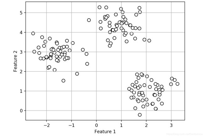
初始数据中心分布:
采用KMeans聚类后,聚类中心分布:
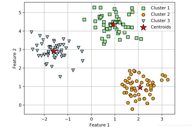
显然,KMeans聚类算法可以较好地将Blob簇分为三类。
第二部分:KMeans算法性能评价
指标一:Elbow
One of the main challenge in unsupervised learning is that we do not know the definite answer.Thus, to quantify the quality of clustering, intrinsic metrics - such as the within-cluster (SSE) distortion - to compare the performance of different k-means clusterings.
Intuitively, if k increases, the distortion will decrease. This is because the samples will be closer to the centroids they are assigned to. The idea behind the elbow method is to identify the value of k where the distortion begins to increase most rapidly, which will be clearer if the distortion for different values k is depicted.
FROM
Sebastian Raschka, Vahid Mirjalili. Python机器学习第二版. 南京:东南大学出版社,2018.
代码
#Section 3: Elbow metric to evaluate model performance
print("Distortion: %.2f" % km.inertia_)

distortions=[]
for i in range(1,11):
    km=KMeans(n_clusters=i,
              init='k-means++',
              n_init=10,
              max_iter=300,
              random_state=0)
    km.fit(X)
    distortions.append(km.inertia_)
plt.plot(range(1,11),distortions,marker='o')
plt.xlabel("Number of Clusters")
plt.ylabel("Distortion")
plt.grid()
plt.savefig("./fig3.png")
plt.show()
值得注意的是,这里“k-means++”的使用是为了避免传统k-means的中心初始化问题。其在于递进选择聚类中心,每更新一个聚类中心,都需采用符合特定概率的分布,以选择和更新聚类中心。
结果
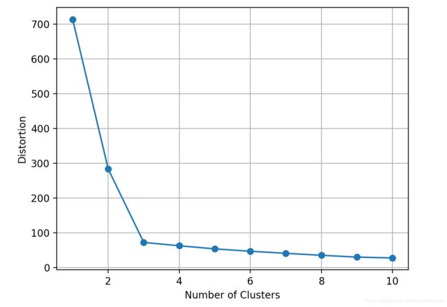
Distortion距离为聚类后,各点与聚类中心的差异总和。换言之,Distortion距离为各类内部距离总和的汇总。
Distortion: 72.48
指标二:Silhouette
Another intrinsic metric to evaluate the quality of a clustering is silhouette analysis, which can also be applied to clustering algorithms other than k-means. Silhouette analysis can be used as a graphical tool to plot a measure of how tightly grouped the samples in the clusters are. To calculate the silhouette coefficient of a single sample in our dataset, its implementation can be summarized in the following three steps:
- Step 1: Calculate the cluster cohesion as the average distance between a sample and all other points in the same cluster
- Step 2: Calculate the cluster sparation from the next closesr cluster as the average distance between the sample and all samples in the nearest cluster
- Step 3: Calculate the silhouette as the difference between cluster cohesion and separation divided by the greater of the two.
Silhouette score: = (separation score-cohesion score)/max(separation score, cohesion score)
Silhouette score is bounded in the range of -1 to 1. The closest to 1, separation score is the largest, which indicates that an ideal silhouette coefficient is obtained, since separation score quantifies how dissimilar a sample is to other clusters and cohesion score tells how similar it is to the other samples in its own cluster.
对比一,聚类数量,设置为3
代码
#Section 4: Silhouette metric to evaluate model performance
#Section 4.1: Set cluster=3
import numpy as np
from matplotlib import cm
from sklearn.metrics import silhouette_score,silhouette_samples

km=KMeans(n_clusters=3,
          init='k-means++',
          n_init=10,
          max_iter=300,
          tol=1e-4,
          random_state=0)
y_km=km.fit_predict(X)

cluster_labels=np.unique(y_km)
n_clusters=cluster_labels.shape[0]
silhouette_score_cluster_3=silhouette_score(X,km.labels_)
print("Silhouette Score When Cluster Number Set to 3: %.3f" % silhouette_score_cluster_3)
silhouette_vals=silhouette_samples(X,y_km,metric='euclidean')
y_ax_lower,y_ax_upper=0,0
yticks=[]
for i,c in enumerate(cluster_labels):
    c_silhouette_vals=silhouette_vals[y_km==c]
    c_silhouette_vals.sort()
    y_ax_upper+=len(c_silhouette_vals)
    color=cm.jet(float(i)/n_clusters)
    plt.barh(range(y_ax_lower,y_ax_upper),
             c_silhouette_vals,
             height=1.0,
             edgecolor='none',
             color=color)
    yticks.append((y_ax_lower+y_ax_upper)/2.0)
    y_ax_lower+=len(c_silhouette_vals)

silhouette_avg=np.mean(silhouette_vals)
plt.axvline(silhouette_avg,
            color='red',
            linestyle='--')
plt.yticks(yticks,cluster_labels+1)
plt.ylabel("Cluster")
plt.xlabel("Silhouette Coefficients")
plt.savefig('./fig4.png')
plt.show()
结果
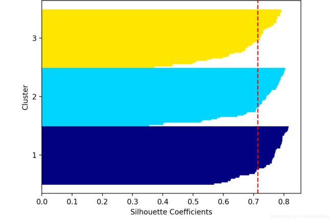
Silhouette分数,如下:
Silhouette Score When Cluster Number Set to 3: 0.714
由上述结果,可以得知平均轮廓系数silhouette趋于0.72左右,亦即类间差异较大,而类内部差异则较小。由此说明,当前设置聚类数量为3,是比较合适的,也与elbow肘系数下降梯度最大为3,是比较契合的。
对比二,聚类数量,设置为2
代码
#Section 4.2: Set cluster=2
import numpy as np
from matplotlib import cm
from sklearn.metrics import silhouette_score,silhouette_samples

km=KMeans(n_clusters=2,
          init='k-means++',
          n_init=10,
          max_iter=300,
          tol=1e-4,
          random_state=0)
y_km=km.fit_predict(X)

cluster_labels=np.unique(y_km)
n_clusters=cluster_labels.shape[0]
silhouette_score_cluster_2=silhouette_score(X,km.labels_)
print("Silhouette Score When Cluster Number Set to 2: %.3f" % silhouette_score_cluster_2)
silhouette_vals=silhouette_samples(X,y_km,metric='euclidean')
y_ax_lower,y_ax_upper=0,0
yticks=[]
for i,c in enumerate(cluster_labels):
    c_silhouette_vals=silhouette_vals[y_km==c]
    c_silhouette_vals.sort()
    y_ax_upper+=len(c_silhouette_vals)
    color=cm.jet(float(i)/n_clusters)
    plt.barh(range(y_ax_lower,y_ax_upper),
             c_silhouette_vals,
             height=1.0,
             edgecolor='none',
             color=color)
    yticks.append((y_ax_lower+y_ax_upper)/2.0)
    y_ax_lower+=len(c_silhouette_vals)

silhouette_avg=np.mean(silhouette_vals)
plt.axvline(silhouette_avg,
            color='red',
            linestyle='--')
plt.yticks(yticks,cluster_labels+1)
plt.ylabel("Cluster")
plt.xlabel("Silhouette Coefficients")
plt.savefig('./fig5.png')
plt.show()
结果
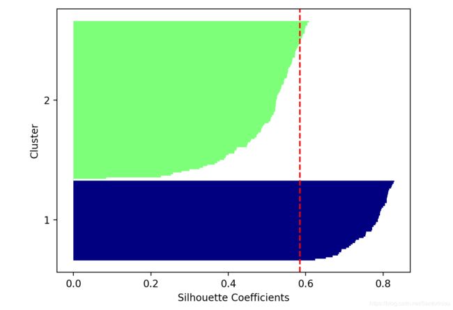
Silhouette分数,如下:
Silhouette Score When Cluster Number Set to 2: 0.585
对比聚类数量设定为3时,聚类中心为2的轮廓系数更低,趋于0.585,亦即类间差异与类内部差异相差幅度不如聚类数量设定为3的结果,由此说明聚类数量设定为2的聚类效果不佳。
FROM
Sebastian Raschka, Vahid Mirjalili. Python机器学习第二版. 南京:东南大学出版社,2018.
参考文献
Sebastian Raschka, Vahid Mirjalili. Python机器学习第二版. 南京:东南大学出版社,2018.
附录
from sklearn import datasets
import matplotlib.pyplot as plt
import warnings
warnings.filterwarnings("ignore")

plt.rcParams['figure.dpi']=200
plt.rcParams['savefig.dpi']=200
font = {'weight': 'light'}
plt.rc("font", **font)

#Section 1: Load Blobs from datasets and visualize it
X,y=datasets.make_blobs(n_samples=150,
                        n_features=2,
                        centers=3,
                        cluster_std=0.5,
                        shuffle=True,
                        random_state=0)
plt.scatter(X[:,0],X[:,1],c='white',marker='o',edgecolors='black',s=50)
plt.grid()
plt.savefig('./fig1.png')
plt.show()

#Section 2: Use KMeans algorithm to visualize data points and centroids
from sklearn.cluster import KMeans

#Set n_init=10 to run k-means clustering algorithm 10 times independently
#with different centroids to choose the final model with the lowest SSE
km=KMeans(n_clusters=3,
          init='random',
          n_init=10,
          max_iter=300,
          tol=1e-4,
          random_state=0)

y_km=km.fit_predict(X)
plt.scatter(X[y_km==0,0],
            X[y_km==0,1],
            s=50,
            c='lightgreen',
            marker='s',
            edgecolor='black',
            label='Cluster 1')
plt.scatter(X[y_km==1,0],
            X[y_km==1,1],
            s=50,
            c='orange',
            marker='o',
            edgecolor='black',
            label='Cluster 2')
plt.scatter(X[y_km==2,0],
            X[y_km==2,1],
            s=50,
            c='lightblue',
            marker='v',
            edgecolor='black',
            label='Cluster 3')
plt.scatter(km.cluster_centers_[:,0],km.cluster_centers_[:,1],
            s=250,
            marker='*',
            c='red',
            edgecolor='black',
            label='Centroids')
plt.xlabel('Feature 1')
plt.ylabel('Feature 2')
plt.legend(loc='best')
plt.grid()
plt.savefig('./fig2.png')
plt.show()

#Section 3: Elbow metric to evaluate model performance
print("Distortion: %.2f" % km.inertia_)

distortions=[]
for i in range(1,11):
    km=KMeans(n_clusters=i,
              init='k-means++',
              n_init=10,
              max_iter=300,
              random_state=0)
    km.fit(X)
    distortions.append(km.inertia_)
plt.plot(range(1,11),distortions,marker='o')
plt.xlabel("Number of Clusters")
plt.ylabel("Distortion")
plt.grid()
plt.savefig("./fig3.png")
plt.show()

#Section 4: Silhouette metric to evaluate model performance
#Section 4.1: Set cluster=3
import numpy as np
from matplotlib import cm
from sklearn.metrics import silhouette_score,silhouette_samples

km=KMeans(n_clusters=3,
          init='k-means++',
          n_init=10,
          max_iter=300,
          tol=1e-4,
          random_state=0)
y_km=km.fit_predict(X)

cluster_labels=np.unique(y_km)
n_clusters=cluster_labels.shape[0]
silhouette_score_cluster_3=silhouette_score(X,km.labels_)
print("Silhouette Score When Cluster Number Set to 3: %.3f" % silhouette_score_cluster_3)
silhouette_vals=silhouette_samples(X,y_km,metric='euclidean')
y_ax_lower,y_ax_upper=0,0
yticks=[]
for i,c in enumerate(cluster_labels):
    c_silhouette_vals=silhouette_vals[y_km==c]
    c_silhouette_vals.sort()
    y_ax_upper+=len(c_silhouette_vals)
    color=cm.jet(float(i)/n_clusters)
    plt.barh(range(y_ax_lower,y_ax_upper),
             c_silhouette_vals,
             height=1.0,
             edgecolor='none',
             color=color)
    yticks.append((y_ax_lower+y_ax_upper)/2.0)
    y_ax_lower+=len(c_silhouette_vals)

silhouette_avg=np.mean(silhouette_vals)
plt.axvline(silhouette_avg,
            color='red',
            linestyle='--')
plt.yticks(yticks,cluster_labels+1)
plt.ylabel("Cluster")
plt.xlabel("Silhouette Coefficients")
plt.savefig('./fig4.png')
plt.show()

#Section 4.2: Set cluster=2
import numpy as np
from matplotlib import cm
from sklearn.metrics import silhouette_score,silhouette_samples

km=KMeans(n_clusters=2,
          init='k-means++',
          n_init=10,
          max_iter=300,
          tol=1e-4,
          random_state=0)
y_km=km.fit_predict(X)

cluster_labels=np.unique(y_km)
n_clusters=cluster_labels.shape[0]
silhouette_score_cluster_2=silhouette_score(X,km.labels_)
print("Silhouette Score When Cluster Number Set to 2: %.3f" % silhouette_score_cluster_2)
silhouette_vals=silhouette_samples(X,y_km,metric='euclidean')
y_ax_lower,y_ax_upper=0,0
yticks=[]
for i,c in enumerate(cluster_labels):
    c_silhouette_vals=silhouette_vals[y_km==c]
    c_silhouette_vals.sort()
    y_ax_upper+=len(c_silhouette_vals)
    color=cm.jet(float(i)/n_clusters)
    plt.barh(range(y_ax_lower,y_ax_upper),
             c_silhouette_vals,
             height=1.0,
             edgecolor='none',
             color=color)
    yticks.append((y_ax_lower+y_ax_upper)/2.0)
    y_ax_lower+=len(c_silhouette_vals)

silhouette_avg=np.mean(silhouette_vals)
plt.axvline(silhouette_avg,
            color='red',
            linestyle='--')
plt.yticks(yticks,cluster_labels+1)
plt.ylabel("Cluster")
plt.xlabel("Silhouette Coefficients")
plt.savefig('./fig5.png')
plt.show()