强化学习学习总结(四)——DQN
一、def
如果我们的state与action很多,就如打砖块游戏,每个时间不同的砖块排列跟剩余都是不同的state,就会导致维度灾难。使用神经网络来 估算 这个 state 的值, 这样就不需要一张表了.
更新方式

二、算法更新
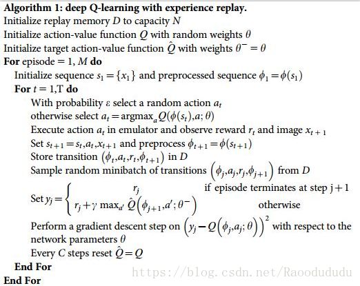
1、初始化replay memory D 容量为N
2、用一个深度神经网络作为Q值网络,初始化权重参数
3、设定游戏片段总数M
4、初始化网络输入,大小为84*84*4,并且计算网络输出
5、以概率ϵ随机选择动作at或者通过网络输出的Q(max)值选择动作at
6、得到执行at后的奖励rt和下一个网络的输入
7、根据当前的值计算下一时刻网络的输出
8、将四个参数作为此刻的状态一起存入到D中(D中存放着N个时刻的状态)
9、随机从D中取出minibatch个状态 (随即采样)
10、计算每一个状态的目标值(通过执行at后的reward来更新Q值作为目标值)
11、通过SGD更新weight

整个算法乍看起来很复杂, 不过我们拆分一下, 就变简单了. 也就是个 Q learning 主框架上加了些装饰.
这些装饰包括:
- 记忆库 (用于重复学习)
- 神经网络计算 Q 值
- 暂时冻结
q_target(现实)参数 (切断相关性)
rom maze_env import Maze
from RL_brain import DeepQNetwork

def run_maze():
    step = 0    # 用来控制什么时候学习
    for episode in range(300):
        # 初始化环境
        observation = env.reset()

        while True:
            # 刷新环境
            env.render()

            # action
            action = RL.choose_action(observation)
            # 获得 state, reward, 是否终止
            observation_, reward, done = env.step(action)
            # DQN 存储记忆
            RL.store_transition(observation, action, reward, observation_)
            # 控制学习起始时间和频率 (先累积一些记忆再开始学习)
            if (step > 200) and (step % 5 == 0):
                RL.learn()
            #  state_ → state
            observation = observation_

            # 如果终止, 就跳出循环
            if done:
                break
            step += 1   # 总步数

    # end of game
    print('game over')
    env.destroy()


if __name__ == "__main__":
    env = Maze()
    RL = DeepQNetwork(env.n_actions, env.n_features,
                      learning_rate=0.01,
                      reward_decay=0.9,
                      e_greedy=0.9,
                      replace_target_iter=200,  # 每 200 步替换一次 target_net 的参数
                      memory_size=2000, # 记忆上限
                      # output_graph=True   # 是否输出 tensorboard 文件
                      )
    env.after(100, run_maze)
    env.mainloop()
    RL.plot_cost()  # 观看神经网络的误差曲线
三、神经网络
暂时冻结q_target参数:方式是搭建两个神经网络, (这两个神经网络结构是完全一样的, 只是里面的参数不一样.)
target_net 用于预测 q_target 值, 他不会及时更新参数. 不可被训练
eval_net 用于预测 q_eval, 这个神经网络拥有最新的神经网络参数. 可被训练

class DeepQNetwork:
    def _build_net(self):
        # -------------- 创建 eval 神经网络, 及时提升参数 --------------
        self.s = tf.placeholder(tf.float32, [None, self.n_features], name='s')  # 用来接收 observation
        self.q_target = tf.placeholder(tf.float32, [None, self.n_actions], name='Q_target') # 用来接收 q_target 的值, 这个之后会通过计算得到
        with tf.variable_scope('eval_net'):
            # c_names(collections_names) 是在更新 target_net 参数时会用到
            c_names, n_l1, w_initializer, b_initializer = \
                ['eval_net_params', tf.GraphKeys.GLOBAL_VARIABLES], 10, \
                tf.random_normal_initializer(0., 0.3), tf.constant_initializer(0.1)  # config of layers

            # eval_net 的第一层. collections 是在更新 target_net 参数时会用到
            with tf.variable_scope('l1'):
                w1 = tf.get_variable('w1', [self.n_features, n_l1], initializer=w_initializer, collections=c_names)
                b1 = tf.get_variable('b1', [1, n_l1], initializer=b_initializer, collections=c_names)
                l1 = tf.nn.relu(tf.matmul(self.s, w1) + b1)

            # eval_net 的第二层. collections 是在更新 target_net 参数时会用到
            with tf.variable_scope('l2'):
                w2 = tf.get_variable('w2', [n_l1, self.n_actions], initializer=w_initializer, collections=c_names)
                b2 = tf.get_variable('b2', [1, self.n_actions], initializer=b_initializer, collections=c_names)
                self.q_eval = tf.matmul(l1, w2) + b2

        with tf.variable_scope('loss'): # 求误差
            self.loss = tf.reduce_mean(tf.squared_difference(self.q_target, self.q_eval))
        with tf.variable_scope('train'):    # 梯度下降
            self._train_op = tf.train.RMSPropOptimizer(self.lr).minimize(self.loss)

        # ---------------- 创建 target 神经网络, 提供 target Q ---------------------
        self.s_ = tf.placeholder(tf.float32, [None, self.n_features], name='s_')    # 接收下个 observation
        with tf.variable_scope('target_net'):
            # c_names(collections_names) 是在更新 target_net 参数时会用到
            c_names = ['target_net_params', tf.GraphKeys.GLOBAL_VARIABLES]

            # target_net 的第一层. collections 是在更新 target_net 参数时会用到
            with tf.variable_scope('l1'):
                w1 = tf.get_variable('w1', [self.n_features, n_l1], initializer=w_initializer, collections=c_names)
                b1 = tf.get_variable('b1', [1, n_l1], initializer=b_initializer, collections=c_names)
                l1 = tf.nn.relu(tf.matmul(self.s_, w1) + b1)

            # target_net 的第二层. collections 是在更新 target_net 参数时会用到
            with tf.variable_scope('l2'):
                w2 = tf.get_variable('w2', [n_l1, self.n_actions], initializer=w_initializer, collections=c_names)
                b2 = tf.get_variable('b2', [1, self.n_actions], initializer=b_initializer, collections=c_names)
                self.q_next = tf.matmul(l1, w2) + b2
四、思维决策
1.代码构架
class DeepQNetwork:
    # 创建神经网络
    def _build_net(self):

    # 初始值
    def __init__(self):

    # 存储记忆
    def store_transition(self, s, a, r, s_):

    # 选行为
    def choose_action(self, observation):

    # 学习
    def learn(self):

    # 看看学习效果 (可选)
    def plot_cost(self):
2.分别实现
(1)创建神经网络
(2)初始值
    def __init__(
            self,
            n_actions,
            n_features,                     #observation数量:如长宽高等
            learning_rate=0.01,
            reward_decay=0.9,
            e_greedy=0.9,
            replace_target_iter=300,        #更新target所间隔的步数
            memory_size=500,                #记忆库记忆容量:记忆上限
            batch_size=32,                  #每次更新所取得记忆数量
            e_greedy_increment=None,        #扩大贪婪率,缩小随机范围,减少探索次数
            output_graph=False,              #出图
    ):
        self.n_actions = n_actions
        self.n_features = n_features
        self.lr = learning_rate
        self.gamma = reward_decay
        self.epsilon_max = e_greedy
        self.replace_target_iter = replace_target_iter
        self.memory_size = memory_size
        self.batch_size = batch_size
        self.epsilon_increment = e_greedy_increment
        self.epsilon = 0 if e_greedy_increment is not None else self.epsilon_max

        # 记录学习次数 (用于判断是否更换 target_net 参数)
        self.learn_step_counter = 0

        # 初始化全 0 记忆 [s, a, r, s_]
        self.memory = np.zeros((self.memory_size, n_features * 2 + 2))      #记忆容量  observation数量+action+reward

        # 创建 [target_net, evaluate_net]
        self._build_net()

        # 替换 target net 的参数
        t_params = tf.get_collection('target_net_params')
        e_params = tf.get_collection('eval_net_params')
        self.replace_target_op = [tf.assign(t, e) for t, e in zip(t_params, e_params)]  # 更新 target_net 参数

        self.sess = tf.Session()

        if output_graph:
            # $ tensorboard --logdir=logs
            # tf.train.SummaryWriter soon be deprecated, use following
            tf.summary.FileWriter("logs/", self.sess.graph)

        self.sess.run(tf.global_variables_initializer())                #初始化所有参数
        self.cost_his = []                                               #记录误差
(3)存储记忆
DQN 的精髓部分之一: 记录下所有经历过的步, 这些步可以进行反复的学习, 所以是一种 off-policy 方法。
 def store_transition(self, s, a, r, s_):
        if not hasattr(self, 'memory_counter'):
            self.memory_counter = 0

        # 记录一条 [s, a, r, s_] 记录
        transition = np.hstack((s, [a, r], s_))
        # 总 memory 大小是固定的, 如果超出总大小, 旧 memory 就被新 memory 迭代更新
        index = self.memory_counter % self.memory_size
        self.memory[index, :] = transition # 替换过程

        self.memory_counter += 1
(4)选行为
    def choose_action(self, observation):
        # to have batch dimension when feed into tf placeholder
        observation = observation[np.newaxis, :]        #转为2维:统一 observation 的 shape (1, size_of_observation)

        if np.random.uniform() < self.epsilon:
            # forward feed the observation and get q value for every actions
            actions_value = self.sess.run(self.q_eval, feed_dict={self.s: observation})
            action = np.argmax(actions_value)
        else:
            action = np.random.randint(0, self.n_actions)
        return action
(5)最重要的一步, 就是在 DeepQNetwork 中, 学习, 更新参数的步骤. 这里涉及了 target_net 和 eval_net 的交互使用.

    def learn(self):
        # 每隔replace_target_iter才更新一次target_net
        if self.learn_step_counter % self.replace_target_iter == 0:
            self.sess.run(self.replace_target_op)
            print('\ntarget_params_replaced\n')

        # 抽取记忆样本
        if self.memory_counter > self.memory_size:
            sample_index = np.random.choice(self.memory_size, size=self.batch_size)
        else:
            sample_index = np.random.choice(self.memory_counter, size=self.batch_size)
        batch_memory = self.memory[sample_index, :]

        #神经网络输出值(输入为memory存储数据)
        q_next, q_eval = self.sess.run(
            [self.q_next, self.q_eval],
            feed_dict={
                self.s_: batch_memory[:, -self.n_features:],  # 存储的后n个features
                self.s: batch_memory[:, :self.n_features],  # 存储的前n个features
            })

        # 将target(现实)值改变为与eval(估计)值位置对应
        # 根据 memory 当中的具体 action 位置来修改 q_target 对应 action 上的值:
        q_target = q_eval.copy()
        batch_index = np.arange(self.batch_size, dtype=np.int32)
        eval_act_index = batch_memory[:, self.n_features].astype(int)
        reward = batch_memory[:, self.n_features + 1]
        q_target[batch_index, eval_act_index] = reward + self.gamma * np.max(q_next, axis=1)

        """
        For example in this batch I have 2 samples and 3 actions:
        q_eval =
        [[1, 2, 3],
         [4, 5, 6]]
        q_target = q_eval =
        [[1, 2, 3],
         [4, 5, 6]]
        Then change q_target with the real q_target value w.r.t the q_eval's action.
        For example in:
            sample 0, I took action 0, and the max q_target value is -1;
            sample 1, I took action 2, and the max q_target value is -2:
        q_target =
        [[-1, 2, 3],
         [4, 5, -2]]
        So the (q_target - q_eval) becomes:
        [[(-1)-(1), 0, 0],
         [0, 0, (-2)-(6)]]
        We then backpropagate this error w.r.t the corresponding action to network,
        leave other action as error=0 cause we didn't choose it.
        """

        # train eval network
        _, self.cost = self.sess.run([self._train_op, self.loss],
                                     feed_dict={self.s: batch_memory[:, :self.n_features],
                                                self.q_target: q_target})
        self.cost_his.append(self.cost)

        # increasing epsilon
        self.epsilon = self.epsilon + self.epsilon_increment if self.epsilon < self.epsilon_max else self.epsilon_max

        self.learn_step_counter += 1
(6)学习效果图
def plot_cost(self):
        import matplotlib.pyplot as plt
        plt.plot(np.arange(len(self.cost_his)), self.cost_his)
        plt.ylabel('Cost')
        plt.xlabel('training steps')
        plt.show()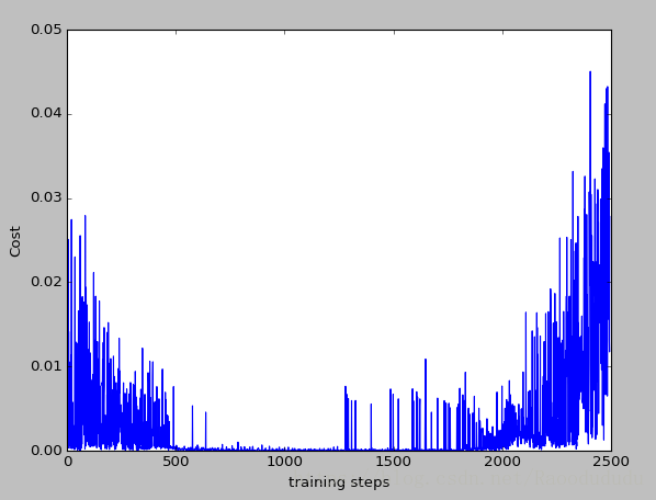
曲线解释:通过探索收集数据,不断有新的数据,所以可能有升高的cost。