理解Logistic回归算法原理与Python实现

一般的机器学习的实现大致都是这样的步骤：
1.准备数据，包括数据的收集，整理等等
2.定义一个学习模型（learning function model），也就是最后要用来去预测其他数据的那个模型
3.定义损失函数（loss function），就是要其做优化那个，以确定模型中参数的那个函数。
4.选择一个优化策略（optimizer），用来根据损失函数不断优化模型的参数。
5.根据训练数据（train data）训练模型（learning function model）
6.根据测试数据（test data）求得模型预测的准确率。

而Logistic回归同样遵循这个步骤，上面的步骤中一，五，六自然是不用说的，剩下的Logistic回归算法与其他的机器学习算法的区别也只在于第二步—学习模型的选择。所以下面主要解释Logistic回归到底确定了一个什么样的模型，然后简单说下损失函数与优化策略。
先来简要介绍一下Logistic回归：**Logistic回归其实只是简单的对特征（feature）做加权相加后结果输入给Sigmoid函数，经过Sigmoid函数后的输出用来确定二分类的结果。**所以Logistic回归的优点在于计算代价不高，容易理解和实现。缺点是很容易造成欠拟合，分类的精度不高。还有一个很重要的地方是神经网络中的一个神经元其实可以理解为一个Logistic回归模型。

Sigmoid函数

首先说下Sigmoid函数，因为它在Logistic回归起着重要的作用，Sigmoid函数是一个在生物学中常见的S型的函数，也称为S型生长曲线。Sigmoid函数由下列公式定义：

下面是两种尺度下的Sigmoid函数图：

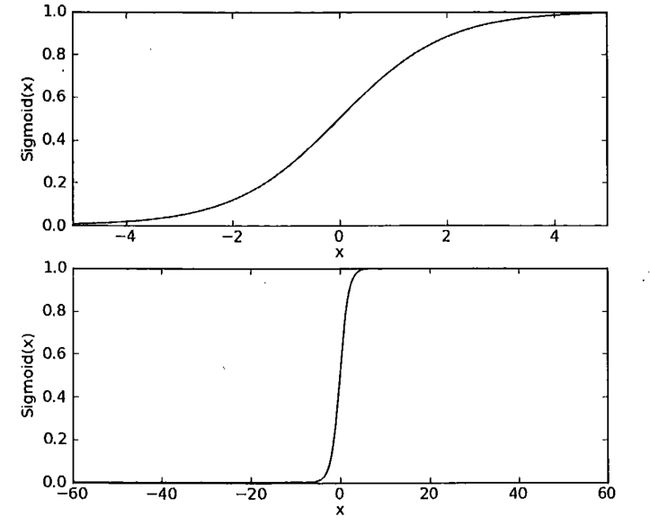
可以看到，在横坐标跨度足够大时，sigmoid函数看起来很像一个阶跃函数。
除此之外，sigmoid函数还有如下特点：
一个良好的阈值函数（最大值趋近于1，最小值趋近于0），连续，光滑，严格单调，且关于(0,0.5)中心对称。

Logistic回归模型##

Logistic回归为了解决二分类问题，需要的是一个这样的函数：函数的输入应当能从负无穷到正无穷，函数的输出0或1。这样的函数很容易让人联想到单位阶跃函数：

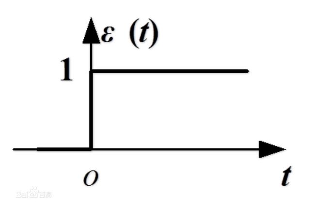
就是上面这个东西，但是单位阶跃函数在跳跃点上从0瞬间跳跃到1，这个瞬间跳跃的过程决定了它并不是连续的，所以它并不是最好的选择，对的，Logistic回归最后选择了上面提到的sigmoid函数。由于sigmoid函数是按照0.5中心对称的，所以只需将它的输出大于0.5的数据作为“1类”，小于0.5的数据作为“0类”，就这样实现了二分类的问题。
确定了sigmoid函数输出怎么处理的问题，那么sigmoid函数的输入又是什么？
其实只是每一个特征（feature）上都乘以一个回归系数，然后把所有的结果值相加，定义sigmoid函数输入为z，那么：

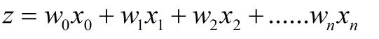
其中就是特征了，而就是需要训练得到的参数。我们都将它用向量的形式表达即为：

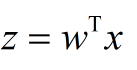
所以Logistic回归模型的形式可以写成：

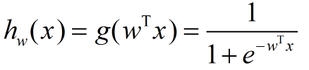
至此，Logistic回归模型就确定好了：

损失函数与优化策略

在上图所示的Logistic回归模型中，激活函数后，阈值函数前的输出为训练模型时需要用到的，在这里设为，其实是一个概率（因为所有的输出都被压缩到0-1之间），所以有时也会用P来表示。而对于一个模型而言，他的损失函数并不是唯一的，对于不同的损失函数可以选用不同的优化策略。

损失函数是在衡量实际的输出与期望输出之间的距离，一般情况下可以使用差平方的方式构建，但是在Logistic回归中往往不使用这种方式，因为这样一来，优化目标不是一个凸函数，在使用梯度下降算法的时候，可能会找到多组最优解。所以在Logistic回归中，一般采用如下定义的loss function。

我们假设y=1时的概率就是，由于是一个二分类问题，那么y=0时的概率就是，我们将取对数并乘上y，最后把所有的样本相加：

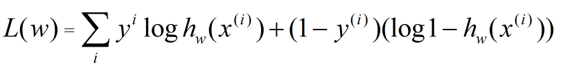
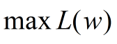
我们希望Logistic回归学习得到参数，能使得正例的特征远大于0，负例的特征远小于0，所以优化问题也就变成了如何去求：

或者：

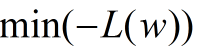
上面上个公式也可以称之为Logistic回归的损失函数（loss function）。

那么对于第一个损失函数，可以采用（随机）梯度上升来作为优化策略，对于第二个损失函数，用（随机）梯度下降就好了。

Python实现

这个例子来源于《机器学习实战》，在这里可以下载电子版。
这个例子使用Logistic回归与随机梯度上升算法来预测病马的生死，下面会贴出源码并简单说明，但是如果想要使用例程中的数据，可以下载整个例程。

from numpy import *

def loadDataSet():
    dataMat = []; labelMat = []
    fr = open('testSet.txt')
    for line in fr.readlines():
        lineArr = line.strip().split()
        dataMat.append([1.0, float(lineArr[0]), float(lineArr[1])])
        labelMat.append(int(lineArr[2]))
    return dataMat,labelMat

def sigmoid(inX):
    return 1.0/(1+exp(-inX))

def gradAscent(dataMatIn, classLabels):
    dataMatrix = mat(dataMatIn)             #convert to NumPy matrix
    labelMat = mat(classLabels).transpose() #convert to NumPy matrix
    m,n = shape(dataMatrix)
    alpha = 0.001
    maxCycles = 500
    weights = ones((n,1))
    for k in range(maxCycles):              #heavy on matrix operations
        h = sigmoid(dataMatrix*weights)     #matrix mult
        error = (labelMat - h)              #vector subtraction
        weights = weights + alpha * dataMatrix.transpose()* error #matrix mult
    return weights

def plotBestFit(weights):
    import matplotlib.pyplot as plt
    dataMat,labelMat=loadDataSet()
    dataArr = array(dataMat)
    n = shape(dataArr)[0] 
    xcord1 = []; ycord1 = []
    xcord2 = []; ycord2 = []
    for i in range(n):
        if int(labelMat[i])== 1:
            xcord1.append(dataArr[i,1]); ycord1.append(dataArr[i,2])
        else:
            xcord2.append(dataArr[i,1]); ycord2.append(dataArr[i,2])
    fig = plt.figure()
    ax = fig.add_subplot(111)
    ax.scatter(xcord1, ycord1, s=30, c='red', marker='s')
    ax.scatter(xcord2, ycord2, s=30, c='green')
    x = arange(-3.0, 3.0, 0.1)
    y = (-weights[0]-weights[1]*x)/weights[2]
    ax.plot(x, y)
    plt.xlabel('X1'); plt.ylabel('X2');
    plt.show()

def stocGradAscent0(dataMatrix, classLabels):
    m,n = shape(dataMatrix)
    alpha = 0.01
    weights = ones(n)   #initialize to all ones
    for i in range(m):
        h = sigmoid(sum(dataMatrix[i]*weights))
        error = classLabels[i] - h
        weights = weights + alpha * error * dataMatrix[i]
    return weights

def stocGradAscent1(dataMatrix, classLabels, numIter=150):
    m,n = shape(dataMatrix)
    weights = ones(n)   #initialize to all ones
    for j in range(numIter):
        dataIndex = range(m)
        for i in range(m):
            alpha = 4/(1.0+j+i)+0.0001    #apha decreases with iteration, does not 
            randIndex = int(random.uniform(0,len(dataIndex)))#go to 0 because of the constant
            h = sigmoid(sum(dataMatrix[randIndex]*weights))
            error = classLabels[randIndex] - h
            weights = weights + alpha * error * dataMatrix[randIndex]
            del(dataIndex[randIndex])
    return weights

def classifyVector(inX, weights):
    prob = sigmoid(sum(inX*weights))
    if prob > 0.5: return 1.0
    else: return 0.0

def colicTest():
    frTrain = open('horseColicTraining.txt'); frTest = open('horseColicTest.txt')
    trainingSet = []; trainingLabels = []
    for line in frTrain.readlines():
        currLine = line.strip().split('\t')
        lineArr =[]
        for i in range(21):
            lineArr.append(float(currLine[i]))
        trainingSet.append(lineArr)
        trainingLabels.append(float(currLine[21]))
    trainWeights = stocGradAscent1(array(trainingSet), trainingLabels, 1000)
    errorCount = 0; numTestVec = 0.0
    for line in frTest.readlines():
        numTestVec += 1.0
        currLine = line.strip().split('\t')
        lineArr =[]
        for i in range(21):
            lineArr.append(float(currLine[i]))
        if int(classifyVector(array(lineArr), trainWeights))!= int(currLine[21]):
            errorCount += 1
    errorRate = (float(errorCount)/numTestVec)
    print "the error rate of this test is: %f" % errorRate
    return errorRate

def multiTest():
    numTests = 10; errorSum=0.0
    for k in range(numTests):
        errorSum += colicTest()
    print "after %d iterations the average error rate is: %f" % (numTests, errorSum/float(numTests))
        

其中定义的函数分别为如下功能：
loadDataSet()：数据准备；
sigmoid():定义sigmoid函数；
gradAscent():梯度上升算法；
plotBestFit():画出决策边界；
stocGradAscent0():随机梯度上升算法；
stocGradAscent1():一种改进的随机梯度上升算法；
classifyVector():一回归系数和特征向量作为输入来计算对应的sigmoid值；
colicTest():打开测试集和训练集，并对数据进行格式化处理；
multiTest():调用colicTest()10次并求结果的平均值。

所以运行上述代码后，在Python提示窗中输入：

>>> import logRegres
>>> reload(logRegres)

>>> logRegres.multiTest()

最后程序输出：

the error rate of this test is: 0.358209
the error rate of this test is: 0.283582
the error rate of this test is: 0.298507
the error rate of this test is: 0.417910
the error rate of this test is: 0.388060
the error rate of this test is: 0.298507
the error rate of this test is: 0.328358
the error rate of this test is: 0.313433
the error rate of this test is: 0.402985
the error rate of this test is: 0.432836
after 10 iterations the average error rate is: 0.352239

0.352239就是最后的错误率了。