ML之K-means：基于K-means算法利用电影数据集实现对top 100 电影进行文档分类

ML之K-means：基于K-means算法利用电影数据集实现对top 100 电影进行文档分类

 

 

 

目录

输出结果

实现代码

---

 

 

 

输出结果

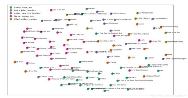
先看文档分类后的结果，一共得到五类电影：

 

实现代码

# -*- coding: utf-8 -*-
from __future__ import print_function

import numpy as np
import pandas as pd
import nltk
from bs4 import BeautifulSoup
import re
import os
import codecs
from sklearn import feature_extraction
import mpld3     #看心情

#import three lists: titles, links and wikipedia synopses
titles = open('document_cluster_master/title_list.txt').read().split('\n')
#ensures that only the first 100 are read in
titles = titles[:100]

links = open('document_cluster_master/link_list_imdb.txt').read().split('\n')
links = links[:100]

synopses_wiki = open('document_cluster_master/synopses_list_wiki.txt').read().split('\n BREAKS HERE')
synopses_wiki = synopses_wiki[:100]

synopses_clean_wiki = []
for text in synopses_wiki:
    text = BeautifulSoup(text, 'html.parser').getText()
    #strips html formatting and converts to unicode
    synopses_clean_wiki.append(text)

synopses_wiki = synopses_clean_wiki
    
    
genres = open('document_cluster_master/genres_list.txt').read().split('\n')
genres = genres[:100]

print(str(len(titles)) + ' titles')
print(str(len(links)) + ' links')
print(str(len(synopses_wiki)) + ' synopses')
print(str(len(genres)) + ' genres')



synopses_imdb = open('document_cluster_master/synopses_list_imdb.txt').read().split('\n BREAKS HERE')
synopses_imdb = synopses_imdb[:100]

synopses_clean_imdb = []

for text in synopses_imdb:
    text = BeautifulSoup(text, 'html.parser').getText()
    #strips html formatting and converts to unicode
    synopses_clean_imdb.append(text)

synopses_imdb = synopses_clean_imdb


synopses = []

for i in range(len(synopses_wiki)):
    item = synopses_wiki[i] + synopses_imdb[i]
    synopses.append(item)
    
    
# generates index for each item in the corpora (in this case it's just rank) and I'll use this for scoring later
#为语料库中的每一个项目生成索引
ranks = []
for i in range(0,len(titles)):
    ranks.append(i)

#定义一些函数对剧情简介进行处理。首先，载入 NLTK 的英文停用词列表。停用词是类似“a”，“the”，或者“in”这些无法传达重要意义的词。我相信除此之外还有更好的解释。
# load nltk's English stopwords as variable called 'stopwords'
stopwords = nltk.corpus.stopwords.words('english')
    
print (stopwords[:10])  #可以查看一下

#接下来我导入 NLTK 中的 Snowball 词干分析器（Stemmer）。词干化（Stemming）的过程就是将词打回原形，其实就是把长得很像的英文单词关联在一起。
# load nltk's SnowballStemmer as variabled 'stemmer'
from nltk.stem.snowball import SnowballStemmer
stemmer = SnowballStemmer("english")


# tokenize_and_stem：对每个词例（token）分词（tokenizes）（将剧情简介分割成单独的词或词例列表）并词干化
# tokenize_only: 分词即可

# 这里我定义了一个分词器（tokenizer）和词干分析器（stemmer），它们会输出给定文本词干化后的词集合
def tokenize_and_stem(text):
    # 首先分句，接着分词，而标点也会作为词例存在
    tokens = [word for sent in nltk.sent_tokenize(text) for word in nltk.word_tokenize(sent)]
    filtered_tokens = []
    # 过滤所有不含字母的词例（例如：数字、纯标点）
    for token in tokens:
        if re.search('[a-zA-Z]', token):
            filtered_tokens.append(token)
    stems = [stemmer.stem(t) for t in filtered_tokens]
    return stems
 
 
def tokenize_only(text):
    # 首先分句，接着分词，而标点也会作为词例存在
    tokens = [word.lower() for sent in nltk.sent_tokenize(text) for word in nltk.word_tokenize(sent)]
    filtered_tokens = []
    # 过滤所有不含字母的词例（例如：数字、纯标点）
    for token in tokens:
        if re.search('[a-zA-Z]', token):
            filtered_tokens.append(token)
    return filtered_tokens

# 使用上述词干化/分词和分词函数遍历剧情简介列表以生成两个词汇表：经过词干化和仅仅经过分词后。

# 非常不 pythonic，一点也不！
# 扩充列表后变成了非常庞大的二维（flat）词汇表
totalvocab_stemmed = []
totalvocab_tokenized = []
for i in synopses:
    allwords_stemmed = tokenize_and_stem(i) #对每个电影的剧情简介进行分词和词干化
    totalvocab_stemmed.extend(allwords_stemmed) # 扩充“totalvocab_stemmed”列表
 
    allwords_tokenized = tokenize_only(i)
    totalvocab_tokenized.extend(allwords_tokenized)
    
#一个可查询的stemm词表，以下是词干化后的词变回原词例是一对多（one to many）的过程：词干化后的“run”能够关联到“ran”，“runs”，“running”等等。
vocab_frame = pd.DataFrame({'words': totalvocab_tokenized}, index = totalvocab_stemmed)
print ('there are ' + str(vocab_frame.shape[0]) + ' items in vocab_frame')
print (vocab_frame.head())

#利用Tf-idf计算文本相似度,利用 tf-idf 矩阵，你可以跑一长串聚类算法来更好地理解剧情简介集里的隐藏结构
from sklearn.feature_extraction.text import TfidfVectorizer

# 定义向量化参数
tfidf_vectorizer = TfidfVectorizer(max_df=0.8, max_features=200000,
                                 min_df=0.2, stop_words='english',
                                 use_idf=True, tokenizer=tokenize_and_stem, ngram_range=(1,3))
tfidf_matrix = tfidf_vectorizer.fit_transform(synopses) # 向量化剧情简介文本
print(tfidf_matrix.shape)                     #(100, 563)，100个电影记录，每个电影后边有563个词

terms = tfidf_vectorizer.get_feature_names()  #terms” 这个变量只是 tf-idf 矩阵中的特征（features）表，也是一个词汇表

#dist 变量被定义为 1 – 每个文档的余弦相似度。余弦相似度用以和 tf-idf 相互参照评价。可以评价全文（剧情简介）中文档与文档间的相似度。被 1 减去是为了确保我稍后能在欧氏（euclidean）平面（二维平面）中绘制余弦距离。
# dist 可以用以评估任意两个或多个剧情简介间的相似度
from sklearn.metrics.pairwise import cosine_similarity
dist = 1 - cosine_similarity(tfidf_matrix)


#1、首先采用k-means算法
#每个观测对象（observation）都会被分配到一个聚类，这也叫做聚类分配（cluster assignment）。这样做是为了使组内平方和最小。接下来，聚类过的对象通过计算来确定新的聚类质心（centroid）。然后，对象将被重新分配到聚类，在下一次迭代操作中质心也会被重新计算，直到算法收敛。
from sklearn.cluster import KMeans

#跑了几次这个算法以后我发现得到全局最优解（global optimum）的几率要比局部最优解（local optimum）大
num_clusters = 5            #需要先设定聚类的数目
km = KMeans(n_clusters=num_clusters)
km.fit(tfidf_matrix)
clusters = km.labels_.tolist()


from sklearn.externals import joblib

joblib.dump(km,  'doc_cluster.pkl')  # 注释语句用来存储你的模型, 因为我已经从 pickle 载入过模型了
km = joblib.load('doc_cluster.pkl')
clusters = km.labels_.tolist()

#进行可视化
import pandas as pd

#创建一个字典，包含片名，排名，简要剧情，聚类分配，还有电影类型（genre）（排名和类型是从 IMDB 上爬下来的）。  为了方便起见，将这个字典转换成了 Pandas DataFrame。
films = { 'title': titles, 'rank': ranks, 'synopsis': synopses, 'cluster': clusters, 'genre': genres }
frame = pd.DataFrame(films, index = [clusters] , columns = ['rank', 'title', 'cluster', 'genre'])
print(frame['cluster'].value_counts())

grouped = frame['rank'].groupby(frame['cluster']) #为了凝聚（aggregation），由聚类分类。
print(grouped.mean())                             #每个聚类的平均排名（1 到 100）,clusters 4 和 clusters 0 的排名最低，说明它们包含的影片在 top 100 列表中相对没那么棒。


#选取n(我选6个)离聚类质心最近的词对聚类进行一些好玩的索引(indexing)和排列(sorting)。这样可以更直观观察聚类的主要主题。
# from __future__ import print_function

print("Top terms per cluster:")
print()
#按离质心的距离排列聚类中心，由近到远
order_centroids = km.cluster_centers_.argsort()[:, ::-1]
for i in range(num_clusters):
    print("Cluster %d words:" % i, end='')
    for ind in order_centroids[i, :6]:  #每个聚类选6个词
        print(' %s' % vocab_frame.ix[terms[ind].split(' ')].values.tolist()[0][0].encode('utf-8', 'ignore'), end=',')
    print()
    print()
    print("Cluster %d titles:" % i, end='')
    for title in frame.ix[i]['title'].values.tolist():
        print(' %s,' % title, end='')
    print()
    print()
    
#This is purely to help export tables to html and to correct for my 0 start rank (so that Godfather is 1, not 0)
frame['Rank'] = frame['rank'] + 1
frame['Title'] = frame['title']
#export tables to HTML
print(frame[['Rank', 'Title']].loc[frame['cluster'] == 1].to_html(index=False))



#此处降维：为了可视化而用，维度太高的数据没法可视化
import os  # for os.path.basename
import matplotlib.pyplot as plt
import matplotlib as mpl
from sklearn.manifold import MDS

MDS()
# two components as we're plotting points in a two-dimensional plane
# "precomputed" because we provide a distance matrix
# we will also specify `random_state` so the plot is reproducible.
mds = MDS(n_components=2, dissimilarity="precomputed", random_state=1)
pos = mds.fit_transform(dist)  # shape (n_components, n_samples)
xs, ys = pos[:, 0], pos[:, 1]

#strip any proper nouns (NNP) or plural proper nouns (NNPS) from a text
from nltk.tag import pos_tag

def strip_proppers_POS(text):
    tagged = pos_tag(text.split()) #use NLTK's part of speech tagger
    non_propernouns = [word for word,pos in tagged if pos != 'NNP' and pos != 'NNPS']
    return non_propernouns


#进行可视化文档聚类
#set up colors per clusters using a dict
cluster_colors = {0: '#1b9e77', 1: '#d95f02', 2: '#7570b3', 3: '#e7298a', 4: '#66a61e'}

#set up cluster names using a dict
cluster_names = {0: 'Family, home, war', 
                 1: 'Police, killed, murders', 
                 2: 'Father, New York, brothers', 
                 3: 'Dance, singing, love', 
                 4: 'Killed, soldiers, captain'}

#create data frame that has the result of the MDS plus the cluster numbers and titles
df = pd.DataFrame(dict(x=xs, y=ys, label=clusters, title=titles)) 

#group by cluster
groups = df.groupby('label')

# set up plot
fig, ax = plt.subplots(figsize=(17, 9)) # set size
ax.margins(0.05) # Optional, just adds 5% padding to the autoscaling

#iterate through groups to layer the plot
#note that I use the cluster_name and cluster_color dicts with the 'name' lookup to return the appropriate color/label
for name, group in groups:
    ax.plot(group.x, group.y, marker='o', linestyle='', ms=12, label=cluster_names[name], color=cluster_colors[name], mec='none')
    ax.set_aspect('auto')
    ax.tick_params(\
        axis= 'x',          # changes apply to the x-axis
        which='both',      # both major and minor ticks are affected
        bottom='off',      # ticks along the bottom edge are off
        top='off',         # ticks along the top edge are off
        labelbottom='off')
    ax.tick_params(\
        axis= 'y',         # changes apply to the y-axis
        which='both',      # both major and minor ticks are affected
        left='off',      # ticks along the bottom edge are off
        top='off',         # ticks along the top edge are off
        labelleft='off')
    
ax.legend(numpoints=1)  #show legend with only 1 point
#add label in x,y position with the label as the film title
for i in range(len(df)):
    ax.text(df.ix[i]['x'], df.ix[i]['y'], df.ix[i]['title'], size=8)  
    
plt.show() #show the plot
#uncomment the below to save the plot if need be
#plt.savefig('clusters_small_noaxes.png', dpi=200)

 

相关文章推荐
Document Clustering with Python

用Python实现文档聚类