Algorithm: Logistic Regression and Gradient Descent

The most classic model in machine learning : Logistic Regression.

Some problems for two class classify

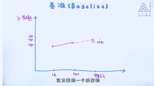
Logistic Regression is a base line for classify problem

When we design a model for machine learning system，at first we create a simple model which is used for the base line and then we optimize the model which will compare with the base line.

A classify problem:

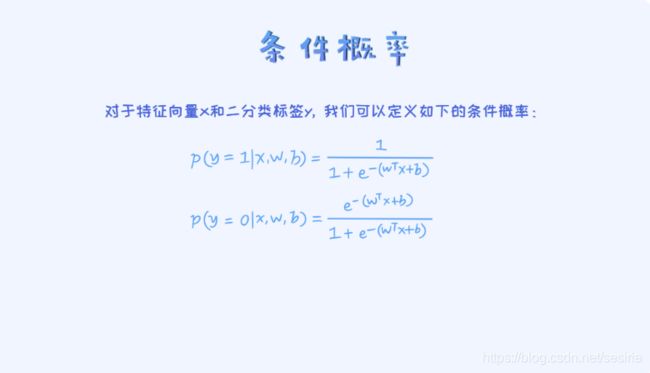
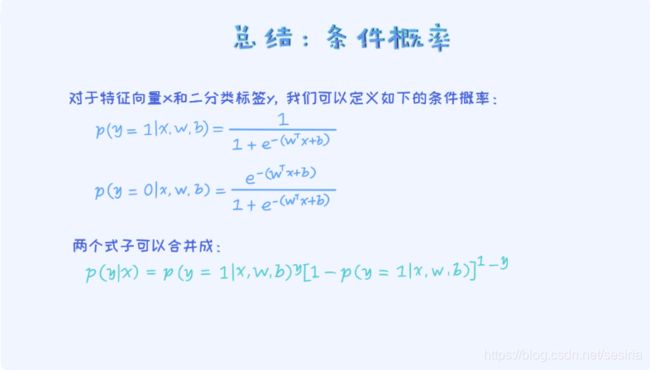
for condition probabiliy: define P(y|x) we need to calculate p(y = 1 |x) and p(y = 0 |x).

For a sample data if p(y = 1 |x) > p(y = 0 |x), we can classify the sample to category '1' ,otherwise '0'.

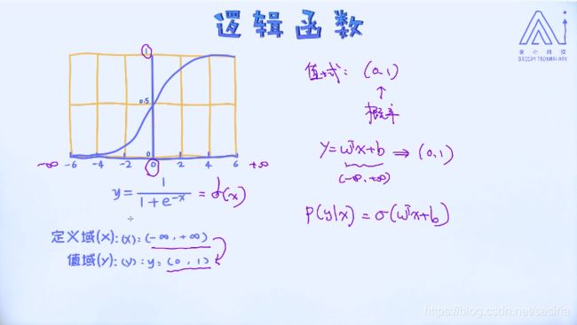
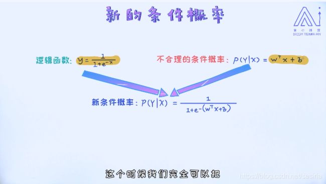
Mapping the linear regression model W.Tx + b into the domain(0,1), sigmoid function:

 

An example:

the condition probability is :

Summary:

Proof for the logistic regression model is an linear model.

decision boundary

 

The loss function for logistic regression:

Maximum Likelihood : for the logistic regression model, there are two parameter as w and b(intercept)

We investigate the input sample data and estimate the maximum of the conditon probability related to the parameters , and maxize this probability to derive the best parameters for the model.

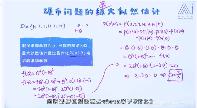
Maximum likelihood estimation:

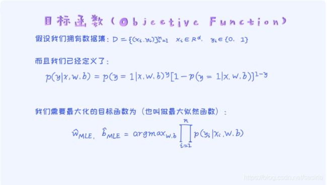
Maximum likelihood for logistic regression:

Xmle = argmax(f(x))  it means that choose the best value of x such that the f(x) is maximum.

Because we assume that the diffrent examples are condition independent. That is P(x1, ..., xn |w) = P(x1|w) * P(x2|w) *...*P(Xn|w)

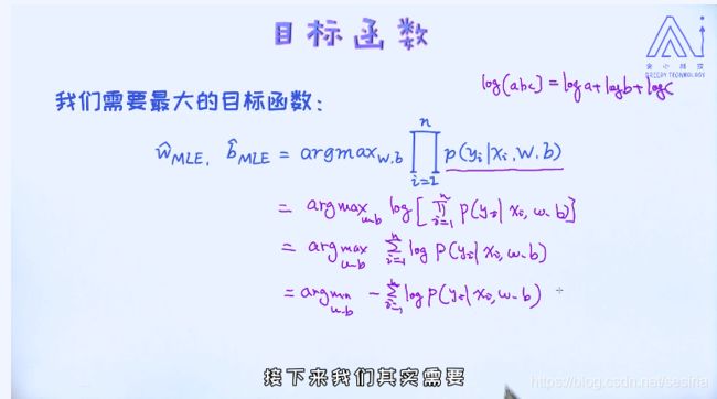
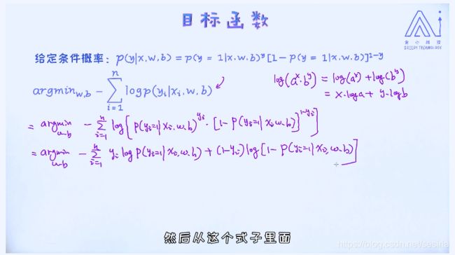
Target function and optimization:

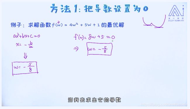
two methods for estimate the max/min value of the function

But some function can't be calculated by setting the first order derivate to zero. such the logistic regression max likelihood function

We need to using the iteration optimization method such as gradient descent.

Learning rate：it controls the speed of the iteration, if it is large then the converge speed is faster, otherwise. But the large learning rate will cause the issue of that the gradient descent can not converge.(diverge)

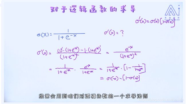
Derivate for sigmoid

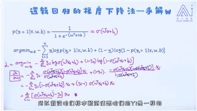
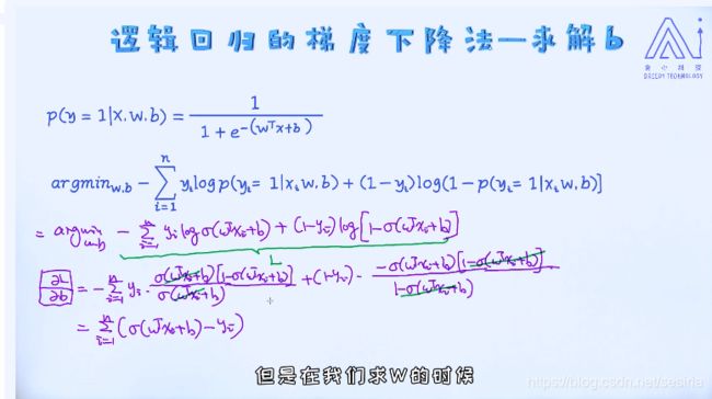
Gradient for target function --w

Gradient for b

 

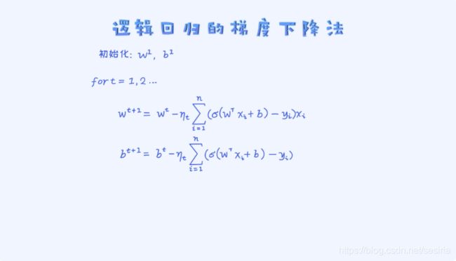
Gradient for logistic Regression:

At first we need to randomize the w and b, and using the iteration to update the w, b

if the target is a convex function, we could get the global optimization, if it is not a convex function we could only get the local optimization.

How to determine that the gradient descent is converge?

Check the value of the cost function(loss function)

 

Logistic Regression implementation:

# import library
import numpy as np
import matplotlib.pyplot as plt
#%matplotlib inline

# generate the data set for classify problem the size is 5000
np.random.seed(12)
num_observations = 5000

x1 = np.random.multivariate_normal([0, 0], [[1, .75], [.75, 1]], num_observations)
x2 = np.random.multivariate_normal([1, 4], [[1, .75], [.75, 1]], num_observations)

X = np.vstack((x1, x2)).astype(np.float32)
y = np.hstack((np.zeros(num_observations),
                np.ones(num_observations)))

print(X.shape, y.shape)

# Data Visualization
plt.figure(figsize = (12, 8))
plt.scatter(X[:, 0], X[:, 1],
            c = y, alpha = .4)
plt.show()

 

 

# sigmoid function
def sigmoid(x):
    return 1 / (1 + np.exp(-x))

# calculate log likelihood
def log_likelihood(X, y, w, b):
    """
    calculate the negative log likelihood, named cross-entropy loss
    the value less, and the performance is better 
    X: training data, N * D
    y: training label,  N * 1
    w: parameter D * 1
    b: bais, which is a scalar
    """

    # get the label related to positive, negative
    pos, neg = np.where(y == 1), np.where(y == 0)

    # calculate the loss for the positive samples.
    pos_sum = np.sum(np.log(sigmoid(X[pos] @ w + b)))

    # calculate the loss for the negative samples.
    neg_sum = np.sum(np.log(1 - sigmoid(X[neg] @ w + b)))

    # return the cross entropy loss
    return -(pos_sum + neg_sum)

# gradient descent for logistic regression
def logistic_regression(X, y, num_steps, learning_rate):
    """
    base on the gradient descent
    X: training data, N * D
    y: training label,  N * 1
    num_steps: iteration times
    learning_rate: size of the step
    """

    w, b = np.zeros(X.shape[1]), 0
    for step in range(num_steps):
        # calculate the error between the predict and the actual
        error = sigmoid(X @ w + b) - y

        # calculate the gradient for w, b
        grad_w = np.matmul(X.T, error)
        grad_b = np.sum(error)

        # update w, b
        w = w - learning_rate * grad_w
        b = b - learning_rate * grad_b

        # calculate the likelihood
        if step % 1000 == 0:
            print(log_likelihood(X, y, w, b))
    
    return w, b

w, b = logistic_regression(X, y, num_steps = 100000, learning_rate = 5e-5)
print("(my) logistic regression with parameter w, b is :", w, b)

# import logisticRegression model from sklearn
from sklearn.linear_model import LogisticRegression

# Set C very large that is it will not add the regular term.
clf = LogisticRegression(fit_intercept = True, C = 1e15)
clf.fit(X, y)

print("(sklearn) logistic regression with parater w, b is :", clf.coef_, clf.intercept_)

 

140.73016092475333
140.72981631073344
140.72949695093567
140.72920097344803
140.7289266473989
140.72867237208226
(my) logistic regression with parameter w, b is : [-5.03280465  8.24664683] -14.017856497489417
d:\ProgramData\Anaconda3\lib\site-packages\sklearn\linear_model\logistic.py:433: FutureWarning: Default solver will be changed to 'lbfgs' in 0.22. Specify a solver to silence this warning.
  FutureWarning)
(sklearn) logistic regression with parater w, b is : [[-5.02712572  8.23286799]] [-13.99400797]

 

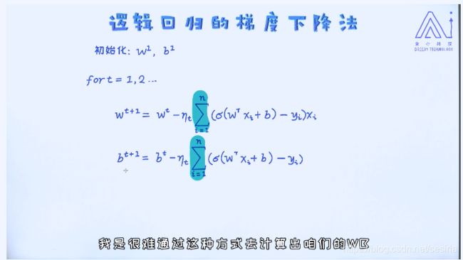
The weakness of Gradient Descent for Logistic Regression

We need to calculate all of the samples for each iteration

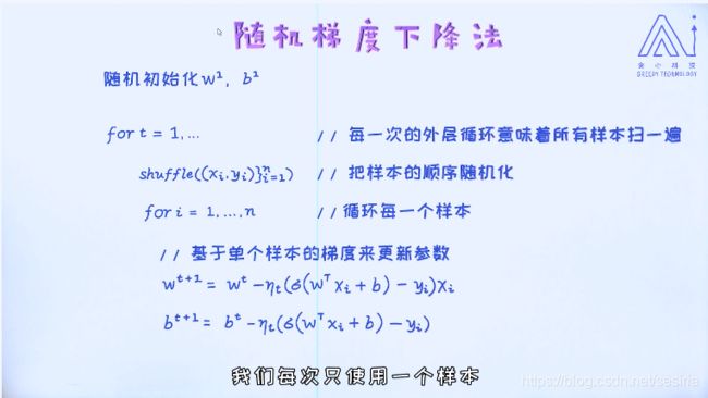
Stochastic Gradient Descent

For each iteration we do not calculate  all of the gradient respect to the samples, we only update 'one' of them.

we don't calculate the sum of the gradient.

Due to that we only use one sample to update the parameter w, there will intro a lot of noise.

In the SGD algorithm, we need to set the learning rate very small. Some update will make our loss function become wose but globally, it will improve our loss function.

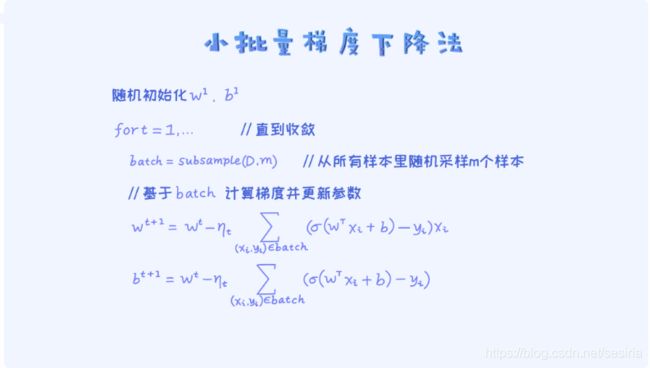
Another approach is the mini-batch gradient descent

 

Logistic Regression mini-batch gradient descent

# logistic Regression by mini-batch gradient descent
# import library
import numpy as np
import matplotlib.pyplot as plt
#%matplotlib inline

# generate the data set for classify problem the size is 5000
np.random.seed(12)
num_observations = 5000

x1 = np.random.multivariate_normal([0, 0], [[1, .75], [.75, 1]], num_observations)
x2 = np.random.multivariate_normal([1, 4], [[1, .75], [.75, 1]], num_observations)

X = np.vstack((x1, x2)).astype(np.float32)
y = np.hstack((np.zeros(num_observations),
                np.ones(num_observations)))

print(X.shape, y.shape)

# Data Visualization
plt.figure(figsize = (12, 8))
plt.scatter(X[:, 0], X[:, 1],
            c = y, alpha = .4)
plt.show()

# sigmoid function
def sigmoid(x):
    return 1 / (1 + np.exp(-x))

# calculate log likelihood
def log_likelihood(X, y, w, b):
    """
    calculate the negative log likelihood, named cross-entropy loss
    the value less, and the performance is better 
    X: training data, N * D
    y: training label,  N * 1
    w: parameter D * 1
    b: bais, which is a scalar
    """

    # get the label related to positive, negative
    pos, neg = np.where(y == 1), np.where(y == 0)

    # calculate the loss for the positive samples.
    pos_sum = np.sum(np.log(sigmoid(X[pos] @ w + b)))

    # calculate the loss for the negative samples.
    neg_sum = np.sum(np.log(1 - sigmoid(X[neg] @ w + b)))

    # return the cross entropy loss
    return -(pos_sum + neg_sum)

# mini-batch gradient descent for logistic regression
def logistic_regression_minibatch(X, y, num_steps, learning_rate):
    """
    base on the gradient descent
    X: training data, N * D
    y: training label,  N * 1
    num_steps: iteration times
    learning_rate: size of the step
    """
    N, D = X.shape
    w, b = np.zeros(X.shape[1]), 0
    for step in range(num_steps):
        # get a random index for minibatch with batch size 100
        index = np.random.choice(range(0, N), 100, replace = False)

        # calculate the error between the predict and the actual
        error = sigmoid(X[index] @ w + b) - y[index]

        # calculate the gradient for w, b
        grad_w = np.matmul(X[index].T, error)
        grad_b = np.sum(error)

        # update w, b
        w = w - learning_rate * grad_w
        b = b - learning_rate * grad_b

        # calculate the likelihood
        if step % 1000 == 0:
            print(log_likelihood(X, y, w, b))
    
    return w, b

w, b = logistic_regression_minibatch(X, y, num_steps = 500000, learning_rate = 5e-4)
print("(my) logistic regression mini-batch with parameter w, b is :", w, b)

# import logisticRegression model from sklearn
from sklearn.linear_model import LogisticRegression

# Set C very large that is it will not add the regular term.
clf = LogisticRegression(fit_intercept = True, C = 1e15, solver = 'lbfgs')
clf.fit(X, y)

print("(sklearn) logistic regression with parater w, b is :", clf.coef_, clf.intercept_)

(my) logistic regression mini-batch with parameter w, b is : [-4.88153788  7.97863031] -13.586978115553702
d:\ProgramData\Anaconda3\lib\site-packages\sklearn\linear_model\logistic.py:433: FutureWarning: Default solver will be changed to 'lbfgs' in 0.22. Specify a solver to silence this warning.
  FutureWarning)
(sklearn) logistic regression with parater w, b is : [[-5.02712572  8.23286799]] [-13.99400797]

 

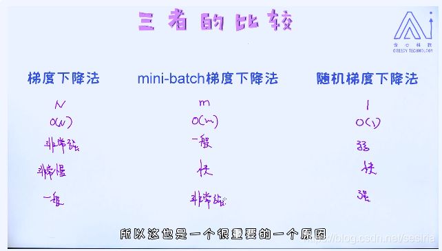
Compare with Gradient Descent, mini-Batch Gradient Descent and Stochastic Gradient Descent

The noise for gradient descent will avoid some saddle point

The saddle point properties of that the gradient is zero but it is not a local optimization.

 

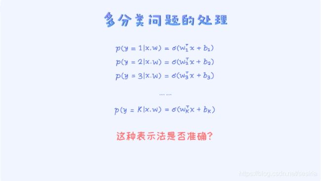
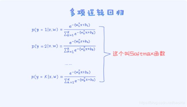
Multinomial Logistic Regression

 

It break the sum rule

Softmax Regression