统计学习方法笔记(六)-非线性支持向量机原理及python实现

非线性支持向量机

定义 非线性支持向量机

从非线性分类训练集，通过核函数与软间隔最大化，或凸二次规划，学习得到的分类决策函数
$$f(x)=\mathrm{sign}\left(\sum _{i=1}^N{\alpha }_i^{\ast }{y}_{i}K\left(x,x_i\right)+b^{\ast }\right)$$
这个分类决策函数称为非线性支持向量机，$K(x,z)$是正定核函数

算法 非线性支持向量机学习算法

输入：训练集$T=\{(x_1,y_1),(x_2,y_2),...,(x_N,y_N)\}$,其中$\mathcal{X}={\mathcal{R}}^n,y_i\in \mathcal{Y}=\{-1,+1\},i=1,2,...,N$;

输出：分类决策函数

第一步：选取适当的核函数$K(x,z)$和适当的参数$C$,构造并求解最优化问题：
$$\underset{\alpha }{\min }\frac{1}{2}\sum _{i=1}^N\sum _{j=1}^N{\alpha }_i{\alpha }_j{y}_i{y}_{j}K\left(x_i\cdot x_j\right)-\sum _{i=1}^N{\alpha }_i$$

$$s.t.\sum _{i=1}^N{\alpha }_i{y}_i=0$$

$$0⩽{\alpha }_i⩽C,i=1,2,\cdots ,N$$

求得最优化问题的解${\alpha }^{\ast }=({\alpha }_1^{\ast },{\alpha }_2^{\ast },\cdots ,{\alpha }_N^{\ast }{)}^T$

第二步：选择${\alpha }^{\ast }$的一个正分量$0<{\alpha }_j^{\ast }<C$,计算
$$b^{\ast }=y_i-\sum _{i=1}^N{\alpha }_i^{\ast }{y}_{i}K(x_i,x_j)$$

第三步：构造决策函数
$$f(x)=\mathrm{sign}\left(\sum _{i=1}^N{\alpha }_i^{\ast }{y}_{i}K(x_i,x_j)\right)$$

注：当$K(x,z)$是正定函数时，(1)、(2)、(3)是凸二次规划问题，存在解。

代码案例 TensorFlow

案例代码已上传：Github地址

import matplotlib.pyplot as plt
import numpy as np
import tensorflow as tf
from sklearn import datasets
from tensorflow.python.framework import ops
ops.reset_default_graph()

sess = tf.Session()

第一步加载数据

# iris.数据 [(Sepal Length, Sepal Width, Petal Length, Petal Width)]
iris = datasets.load_iris()
x_vals = np.array([[x[0], x[3]] for x in iris.data])
y_vals = np.array([1 if y==0 else -1 for y in iris.target])
class1_x = [x[0] for i,x in enumerate(x_vals) if y_vals[i]==1]
class1_y = [x[1] for i,x in enumerate(x_vals) if y_vals[i]==1]
class2_x = [x[0] for i,x in enumerate(x_vals) if y_vals[i]==-1]
class2_y = [x[1] for i,x in enumerate(x_vals) if y_vals[i]==-1]

第二步：声明模型变量并设置损失函数

# 批量大小
batch_size = 150

# 初始化占位符
x_data = tf.placeholder(shape=[None, 2], dtype=tf.float32)
y_target = tf.placeholder(shape=[None, 1], dtype=tf.float32)
prediction_grid = tf.placeholder(shape=[None, 2], dtype=tf.float32)

# 创建变量
b = tf.Variable(tf.random_normal(shape=[1,batch_size]))

本案例采用高斯核函数，将低维空间数据转换为高维空间数据
$$K(x,x^{\prime })=exp\left(-\gamma ||x-x^{\prime }|{|}^2\right)$$

损失函数：
$$-\left(\sum \text{b}-\sum \left(K\cdot ||\text{b}|{|}^2||\text{y}|{|}^2\right)\right)$$

# 高斯核函数 (RBF) 
gamma = tf.constant(-50.0)
sq_vec = tf.multiply(2., tf.matmul(x_data, tf.transpose(x_data)))
my_kernel = tf.exp(tf.multiply(gamma, tf.abs(sq_vec)))

# SVM模型的损失函数
first_term = tf.reduce_sum(b)
b_vec_cross = tf.matmul(tf.transpose(b), b)
y_target_cross = tf.matmul(y_target, tf.transpose(y_target))
second_term = tf.reduce_sum(tf.multiply(my_kernel, tf.multiply(b_vec_cross, y_target_cross)))
loss = tf.negative(tf.subtract(first_term, second_term))

声明预测时所采用的的核函数 RBF

rA = tf.reshape(tf.reduce_sum(tf.square(x_data), 1),[-1,1])
rB = tf.reshape(tf.reduce_sum(tf.square(prediction_grid), 1),[-1,1])
pred_sq_dist = tf.add(tf.subtract(rA, tf.multiply(2., tf.matmul(x_data, tf.transpose(prediction_grid)))), tf.transpose(rB))
pred_kernel = tf.exp(tf.multiply(gamma, tf.abs(pred_sq_dist)))

prediction_output = tf.matmul(tf.multiply(tf.transpose(y_target),b), pred_kernel)
prediction = tf.sign(prediction_output-tf.reduce_mean(prediction_output))
accuracy = tf.reduce_mean(tf.cast(tf.equal(tf.squeeze(prediction), tf.squeeze(y_target)), tf.float32))

优化器设置

# 优化器的设置
my_opt = tf.train.GradientDescentOptimizer(0.01)
train_step = my_opt.minimize(loss)

# 初始化变量
init = tf.global_variables_initializer()
sess.run(init)

第三步：训练

# 开始训练
loss_vec = []
batch_accuracy = []
for i in range(300):
    rand_index = np.random.choice(len(x_vals), size=batch_size)
    rand_x = x_vals[rand_index]
    rand_y = np.transpose([y_vals[rand_index]])
    sess.run(train_step, feed_dict={x_data: rand_x, y_target: rand_y})
    
    temp_loss = sess.run(loss, feed_dict={x_data: rand_x, y_target: rand_y})
    loss_vec.append(temp_loss)
    
    acc_temp = sess.run(accuracy, feed_dict={x_data: rand_x,
                                             y_target: rand_y,
                                             prediction_grid:rand_x})
    batch_accuracy.append(acc_temp)
    
    if (i+1)%75==0:
        print('迭代次数#' + str(i+1))
        print('损失 = ' + str(temp_loss))

绘制图

# Create a mesh to plot points in
x_min, x_max = x_vals[:, 0].min() - 1, x_vals[:, 0].max() + 1
y_min, y_max = x_vals[:, 1].min() - 1, x_vals[:, 1].max() + 1
xx, yy = np.meshgrid(np.arange(x_min, x_max, 0.02),
                     np.arange(y_min, y_max, 0.02))
grid_points = np.c_[xx.ravel(), yy.ravel()]
[grid_predictions] = sess.run(prediction, feed_dict={x_data: x_vals,
                                                   y_target: np.transpose([y_vals]),
                                                   prediction_grid: grid_points})
grid_predictions = grid_predictions.reshape(xx.shape)

%matplotlib inline
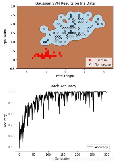
# Plot points and grid
plt.contourf(xx, yy, grid_predictions, cmap=plt.cm.Paired, alpha=0.8)
plt.plot(class1_x, class1_y, 'ro', label='I. setosa')
plt.plot(class2_x, class2_y, 'kx', label='Non setosa')
plt.title('Gaussian SVM Results on Iris Data')
plt.xlabel('Petal Length')
plt.ylabel('Sepal Width')
plt.legend(loc='lower right')
plt.ylim([-0.5, 3.0])
plt.xlim([3.5, 8.5])
plt.show()

# Plot batch accuracy
plt.plot(batch_accuracy, 'k-', label='Accuracy')
plt.title('Batch Accuracy')
plt.xlabel('Generation')
plt.ylabel('Accuracy')
plt.legend(loc='lower right')
plt.show()

案例地址

案例代码已上传：Github地址

参考资料：
[1] 《统计学习方法》
[2]: 《TensorFlow machine learning cookbook》

Github地址https://github.com/Vambooo/lihang-dl

更多技术干货在公众号：深度学习学研社