机器学习系列之coursera week 3 Logistic Regression

目录

1. Classification and Representation

1.1 Classification

1.2 Hypothesis representation of Logistic Regression

1.3 Decision boundary

2. Logistic Regression Model

2.1 Cost function

2.2 Simplified cost function and gradient descent

2.3 Advanced optimization

3. Multiclass classification: one-vs-all

4. Solving the problem of overfitting

4.1 The problem of overfitting

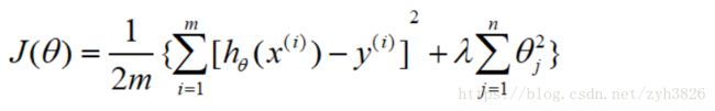
4.2 Cost function

4.3 Regularized Linear Regression

4.4 Regularized Logistic Regression

---

1. Classification and Representation

1.1 Classification

classifiction:

Email: Spam / not spam

online transaction: Fraudulent(yes/no) 欺骗性的

tumor: Malignant / benign

0: negative class

1: positive class

e.g.

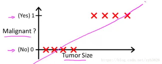图1

(引自coursera week2 Classification)

threshold classifier output h(x) at 0.5

If h(x) >= 0.5, predict y = 1

If h(x) < 0.5, predict y = 0

但是加入一个样本点后， 如图2蓝色直线：

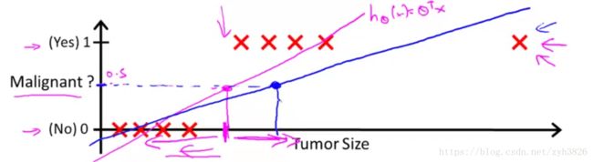图2

(引自coursera week2 Classification)

这会导致分类错误，因此线性回归一般不会用于分类

use linear regression, h(x) may > 1 or < 0

Logistic regression: 0 <= h(x) <= 1

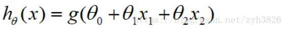
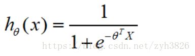
1.2 Hypothesis representation of Logistic Regression

Logistic Regression model:

want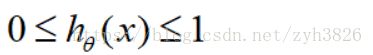

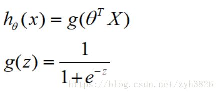
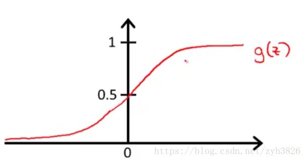图3

(引自coursera week2 hypothesis represention)

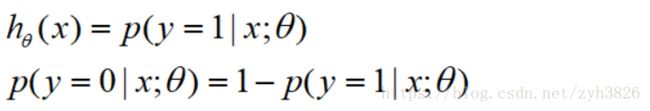
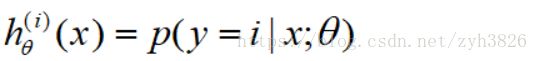
Interpretation of hypothesis output:

 = estimated probability that y=1 on input x

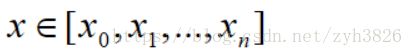
e.g. if x = [x0; x1] = [1; tumor size]

h(x) = 0.7 tell patient that 70% chance of tumor being malignant

1.3 Decision boundary

Logistic Regression:

suppose:  predict y=1, if h(x)>=0.5, 

 predict y=0, if h(x)<=0.5,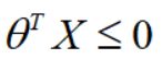 

Decision boundary:

suppose θ0 = -3, θ1 = 1, θ2 = 1

predict y = 1, if -3 + x1 + x2 >= 0, 即 x1 + x2 >= 3, decision boundary 如图4：

图4

(引自coursera week2 decision boundary)

Non-linear decision boundary:

由多项式回归的思想可对h(x)添加高阶项:

suppose:

θ0 = -1, θ1 = 0, θ2 = 0, θ3 = 1, θ4 = 1

predict y=1, if -1 + x1^2 + x2^2 >= 0, 即 x1^2 + x2^2 >= 1, 如图4：

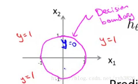图5

(引自coursera week2 decision boundary)

 

2. Logistic Regression Model

2.1 Cost function

Training set:  

x0 = 1, y = {0, 1}

how to choose θ？

Cost function:

因为h(x)为sigmoid函数，若使用

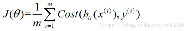
则J(θ)为非凸函数，运用Gradient Descent不能保证能找到全局最小值。

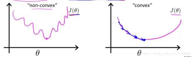图6

(引自coursera week2 Cost Function)

Logistic regression cost function"

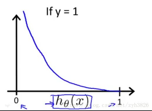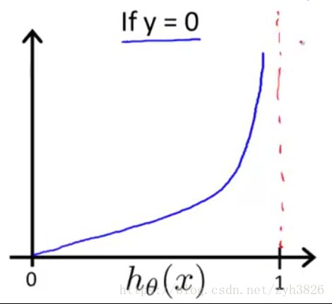图7图8

(引自coursera week2 Cost Function)

2.2 Simplified cost function and gradient descent

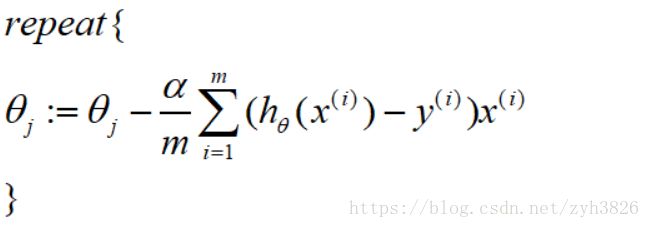
LR cost function:

simplified:

To fit parameters θ:

Gradient descent:

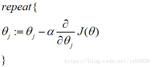
(simultaneously update all θj)

即：

2.3 Advanced optimization

cost function J(θ), want minJ(θ)

Given θ, we have code that can comput:

-J(θ)

-partial derivative of J(θ)

advanced optimization algorithm:

-Conjugate gradient

-BFGS

-L-BFGS

advantages:

-NO need to manually pick α

-ofen faster than gradient descent

disadvantages:

-more complex

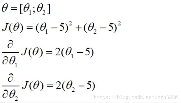
code:

function [jVal, grad] = costFunction(theta)
	jVal = (theta(1) - 5)^2 + (theta(2)-5)^2;
	grad = zeros(2, 1);
	grad(1) = 2 * (theta(1) - 5);
	grad(2) = 2 * (theta(2) - 5);
end

options = optimset('GradObj', 'on', 'MaxIter', 100);
initialTheta = zeros(2, 1);
[optTheta, functionVal, excitFlag] = fminunc(@costFunction, initialTheta, options);

 

3. Multiclass classification: one-vs-all

One-vs-all(One-vs-rest):如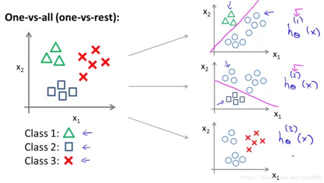图9

图9

(引自coursera week2 Multiclass Classification)

共得到如上图的三个分类器。

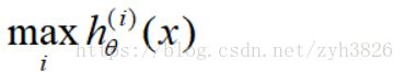
on a new input x, to make a prediction, pick the class i that maximizes:

 

4. Solving the problem of overfitting

4.1 The problem of overfitting

E.g. Linear regression (housing prices)

图10

(引自coursera week2 The problem of overfitting)

图10中第一个图为underfitting(high bias)，第三个图为overfitting(high variance)

addressing overfitting:

options:

(1) Reduce number of features

-Manually select which features to keep

-Model selecting algorithm

(2) Regularization

-keep all the features, but reduce magnitude/values of parameters θ, works well when we have a lot of features, each of which contributes a bit to predict y.

4.2 Cost function

Intuition

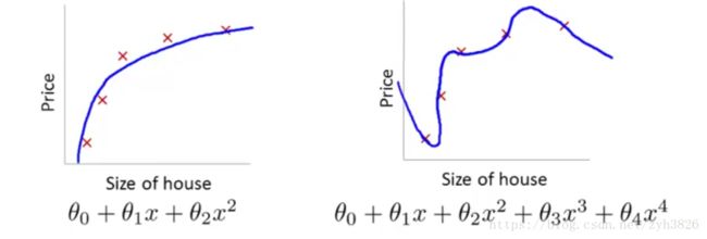图11

(引自coursera week2 Cost function)

suppose we penalize and make θ3, θ4 really small

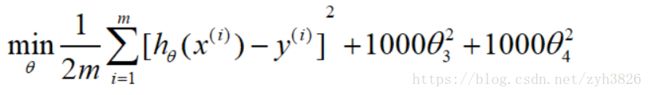
这能使θ3, θ4尽可能的小，θ3, θ4约等于0

Regularization

small values for parameters θ0, θ1, ... ,θn

-"simpler" hypothesis

-Less prone to overfitting

for linear regression:

housing:

-features: x1, x2, ... x100

-parameters: θ0, θ1, ... ,θ100

特别注意：一般不惩罚θ0

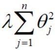称为正则化项，λ为正则化参数

λ的作用：（1）保持训练目的，即最小化损失函数；（2）保持参数较小

Q：为什么λ设置极端大后，会导致欠拟合

对参数惩罚太重会导致θj约等于0， 进而h(x)约等于θ0，即欠拟合

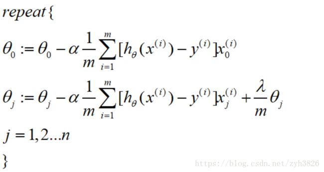
4.3 Regularized Linear Regression

Gradient descent:

normal equation:

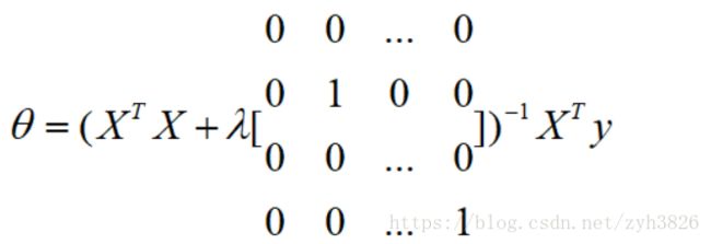
当m不可逆，但上式可逆。

4.4 Regularized Logistic Regression

cost function:

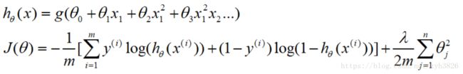
Gradient descent: