线性回归

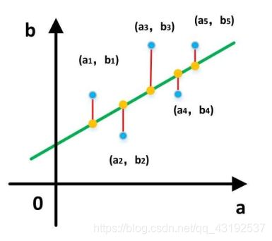
• 一元线性回归

通常当数据只有一个特征时，可表示函数为 f(x) = wx + b，但是实际的数据可能有多个特征，那么这时就可以表示为多元函数了，但是我们现在只考虑一元函数的求解

这里的f(x) 和 x都是已知的，且有多组，未知的是w,b，这正是我们要求解的，以下我们用最小二乘法求解

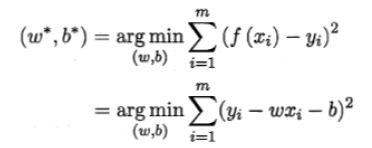
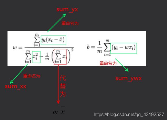
• 最小二乘法求解思想

各个点到直线的欧式距离的平方和的最小时，求此时函数的偏导数，并将偏导数等0所计算出来的w和b，就是我们要求解的

注意：不是点到直线的距离

上述可简单归纳为

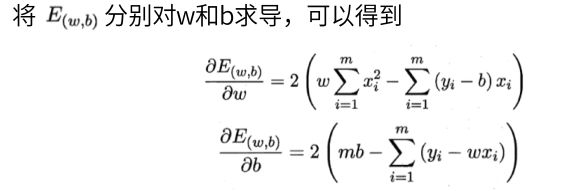
然后求偏导

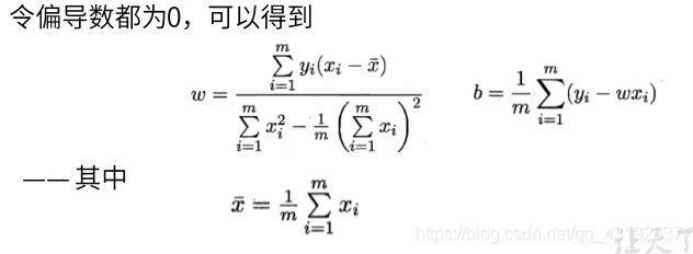
令偏导为0

• 用代码求解w b

data.csv是一系列的x y坐标

数据下载

• jupyter notebook

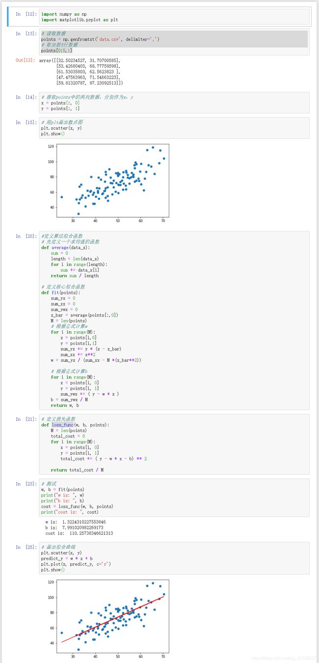
• 源码

import numpy as np
import matplotlib.pyplot as plt

# 读取数据
points = np.genfromtxt('data.csv', delimiter=',')
# 取出前5行数据
points[0:5,:]

# 提取points中的两列数据，分别作为x，y
x = points[:, 0]
y = points[:, 1]

# 用plt画出散点图
plt.scatter(x, y)
plt.show()

#定义算法拟合函数
# 先定义一个求均值的函数
def average(data_x):
    sum = 0
    length = len(data_x)
    for i in range(length):
        sum += data_x[i]
    return sum / length

# 定义核心拟合函数
def fit(points):
    sum_yx = 0
    sum_xx = 0
    sum_ywx = 0
    x_bar = average(points[:,0])
    M = len(points)
    # 根据公式计算w
    for i in range(M):
        x = points[i,0]
        y = points[i,1]
        sum_yx += y * (x - x_bar)
        sum_xx += x**2
    w = sum_yx / (sum_xx - M *(x_bar**2))
    
    # 根据公式计算b
    for i in range(M):
        x = points[i, 0]
        y = points[i, 1]
        sum_ywx += ( y - w * x )
    b = sum_ywx / M
    return w, b

# 定义损失函数
def loss_func(w, b, points):
    M = len(points)
    total_cost = 0
    for i in range(M):
        x = points[i, 0]
        y = points[i, 1]
        total_cost += ( y - w * x - b) ** 2
       
    return total_cost / M

# 测试
w, b = fit(points)
print("w is: ", w)
print("b is: ", b)
cost = loss_func(w, b, points)
print("cost is: ", cost)

# 画出拟合曲线
plt.scatter(x, y)
predict_y = w * x + b
plt.plot(x, predict_y, c='r')
plt.show()

• sklearn库实现求w b

• jupyter notebook

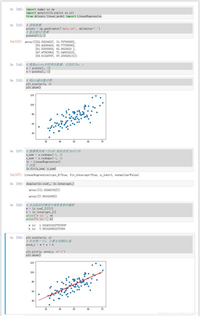
• 源码

import numpy as np
import matplotlib.pyplot as plt
from sklearn.linear_model import LinearRegression

# 读取数据
points = np.genfromtxt('data.csv', delimiter=',')
# 取出前5行数据
points[0:5,:]

# 提取points中的两列数据，分别作为x，y
x = points[:, 0]
y = points[:, 1]

# 用plt画出散点图
plt.scatter(x, y)
plt.show()

# 数据原来是一行n列 现在改变为n行1列
x_new = x.reshape(-1, 1)
y_new = y.reshape(-1, 1)
lr = LinearRegression()
# 训练
lr.fit(x_new, y_new)

display(lr.coef_, lr.intercept_)

# 从训练好的模型中提取系数和截距
w = lr.coef_[0][0]
b = lr.intercept_[0]
print("w is: ", w)
print("b is: ", b)

plt.scatter(x, y)
# 针对每一个x，计算出预测的y值
pred_y = w * x + b

plt.plot(x, pred_y, c='r')
plt.show()

• 梯度下降求解线性回归

梯度就是函数的变化率，变化率也就是函数的导数，当函数的变化率不在改变时，也就意味着导数为0

import numpy as np

points = np.genfromtxt('../data/data.csv',delimiter=',')
points[0:5,:]
X = points[:,0]
y = points[:,1]
class Linear_model(object):
    def __init__(self):
        self.w = np.random.randn(1)[0]
        self.b = np.random.randn(1)[0]
        
    # 模型函数
    def model(self, x):
        return self.w * x + self.b
     ，
    def loss(self,x, y):
        # 求w和b求偏导
        g_w = 2 * (y - self.model(x))*(-x)
        
        g_b = 2 * (y - self.model(x))*(-1)
        return g_w, g_b
    
    def gradient_descend(self,g_w, g_b, step = 0.01):
        self.w = self.w - g_w * step
        self.b = self.b - g_b * step
        
    
    def fit(self,X, y):
        w_last = self.w + 1
        b_last = self.b + 1
        precision = 0.00001
        max_count = 200
        count = 0
        while True:
            if(np.abs(self.w - w_last) < precision) and (np.abs(self.b - b_last) < (precision)):
                break
            if count > max_count:
                break
            size = X.shape[0]
            g_w = 0
            g_b = 0
            # 将所有点代入到此时的w和b对应的偏导数中，累加后，求出所有点的偏导数的平均值   
            for xi, yi in zip(X, y):
                g_w += self.loss(xi, yi)[0] / size
                g_b += self.loss(xi, yi)[1] / size
            self.gradient_descend(g_w, g_b)
            count += 1
            
    def coef_(self):
        return self.w
    
    def intercept_(self):
        return self.b
lm = Linear_model()
# X数据必须是二维的 y可以是二维的，也可以是一维的
# 如果y是二维的，coef_也是二维的
# 如果y是一维的，coef_也是一维的
lm.fit(X.reshape(-1, 1),y)
display(lm.coef_(),lm.intercept_())