图像检索
图像检索
- Bag Of Features 图像检索
- 原理
- Bag of Words 模型
- Bag of Feature算法
- 步骤
- 实验
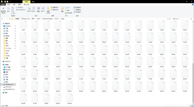
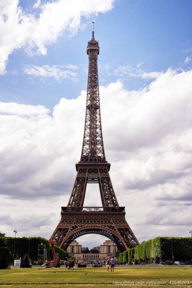
- 1、构造100张图片的数据集
- 2、对所有图片进行SIFT特征提取
- 代码
- 实验结果
- 3、采用k-means算法学习“视觉词典”
- 代码
- 实验结果
- 4、根据IDF计算每个视觉单词的权,并保存至数据库
- 代码
- 实验结果
- 5、图像索引测试
- 代码
- 实验结果
- 实验结论
Bag Of Features 图像检索
原理
Bag of features(Bof)一种是用于图像和视频检索的算法,此算法的神奇之处,就在于对于不同角度,光照的图像,基本都能在图像库中正确检索。
Bag of Words 模型
要了解「Bag of Feature」,首先要知道「Bag of Words」。
「Bag of Words」 是文本分类中一种通俗易懂的策略。一般来讲,如果我们要了解一段文本的主要内容,最行之有效的策略是抓取文本中的关键词,根据关键词出现的频率确定这段文本的中心思想。
比如:如果一则新闻中经常出现「iraq」、「terrorists」,那么,我们可以认为这则新闻应该跟伊拉克的恐怖主义有关。而如果一则新闻中出现较多的关键词是「soviet」、「cuba」,我们又可以猜测这则新闻是关于冷战的(见下图)。

「Bag of words」中的 words ,它们是区分度较高的单词。根据这些 words ,我们就可以快速识别出文章内容,并对文章进行分类。
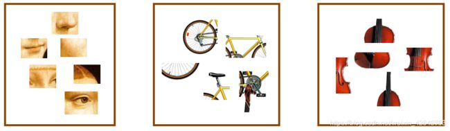
而「Bag of Feature」算法与其大同小异,只是我们抽出的“关键词word”是图像中的关键特征。
Bag of Feature算法
首先我们要找到图像中的关键词,而且这些关键词必须具备较高的区分度。实际过程中,通常会采用SIFT特征。
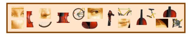
特征聚类:
提取完特征后,我们会采用一些聚类算法对这些特征向量进行聚类。最常用的聚类算法是 k-means。至于 k-means 中的 k 如何取,要根据具体情况来确定。另外,由于特征的数量可能非常庞大,这个聚类的过程也会非常漫长。
聚类完成后,我们就得到了这 k 个向量组成的视觉词典。
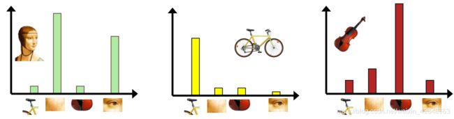
转化直方图:
上一步训练得到的字典,是为了这一步对图像特征进行量化。对于一幅图像而言,我们可以提取出大量的SIFT特征点,但这些特征点仍然缺乏代表性。因此,这一步的目标,是根据字典重新提取图像的高层特征。
具体做法是,对于图像中的每一个SIFT特征,都可以在字典中找到一个最相似的 ,这样,我们可以统计一个 k 维的直方图,代表该图像的SIFT特征在字典中的相似度频率。
步骤
1、用sift算法生成图像库中每幅图的特征点及描述符。
2、再用k-means算法对图像库中的特征点进行聚类,得到一部视觉词典。
3、针对输入特征集,根据视觉词典进行量化
4、把输入图像转化成视觉单词(visual words) 的频率直方图
5、构造特征到图像的倒排表,通过倒排表快速 索引相关图像
6、根据索引结果进行直方图匹配
实验
1、构造100张图片的数据集
2、对所有图片进行SIFT特征提取
代码
from PIL import Image
from pylab import *
from PCV.localdescriptors import sift

from matplotlib.font_manager import FontProperties
font = FontProperties(fname=r"c:\windows\fonts\SimSun.ttc", size=14)

for i in range(100):
    imname = 'data/' + str(i + 1) + '.jpg'
    im = array(Image.open(imname).convert('L'))
    sift.process_image(imname, 'data/' + str(i + 1) + '.sift')
实验结果
3、采用k-means算法学习“视觉词典”
代码
# -*- coding: utf-8 -*-
import pickle
from PCV.imagesearch import vocabulary
from PCV.tools.imtools import get_imlist
from PCV.localdescriptors import sift

#获取图像列表
imlist = get_imlist('first1000/')
nbr_images = len(imlist)
#获取特征列表
featlist = [imlist[i][:-3]+'sift' for i in range(nbr_images)]

#提取文件夹下图像的sift特征
for i in range(nbr_images):
    sift.process_image(imlist[i], featlist[i])

#生成词汇
voc = vocabulary.Vocabulary('ukbenchtest')
voc.train(featlist, 1000, 10)
#保存词汇
# saving vocabulary
with open('first1000/vocabulary.pkl', 'wb') as f:
    pickle.dump(voc, f)
print ('vocabulary is:', voc.name, voc.nbr_words)
实验结果
4、根据IDF计算每个视觉单词的权,并保存至数据库
代码
# -*- coding: utf-8 -*-
import pickle
from PCV.imagesearch import imagesearch
from PCV.localdescriptors import sift
from sqlite3 import dbapi2 as sqlite
from PCV.tools.imtools import get_imlist

#获取图像列表
imlist = get_imlist('first1002/')
nbr_images = len(imlist)
#获取特征列表
featlist = [imlist[i][:-3]+'sift' for i in range(nbr_images)]

# load vocabulary
#载入词汇
with open('first1002/vocabulary.pkl', 'rb') as f:
    voc = pickle.load(f)
#创建索引
indx = imagesearch.Indexer('testImaAdd3.db',voc)
indx.create_tables()
# go through all images, project features on vocabulary and insert
    #遍历所有的图像,并将它们的特征投影到词汇上
for i in range(nbr_images)[:1000]:
    locs,descr = sift.read_features_from_file(featlist[i])
    indx.add_to_index(imlist[i],descr)
# commit to database
#提交到数据库
indx.db_commit()

con = sqlite.connect('testImaAdd3.db')
print (con.execute('select count (filename) from imlist').fetchone())
print (con.execute('select * from imlist').fetchone())
实验结果
得到一个数据库文件testmaAdd
![]()
5、图像索引测试
代码
# -*- coding: utf-8 -*-

import pickle

import sift

from PCV.imagesearch import imagesearch

from PCV.geometry import homography

from PCV.tools.imtools import get_imlist

# load image list and vocabulary

# 载入图像列表

imlist = get_imlist('D:/Python/ComputerView/test1/first1000/')

nbr_images = len(imlist)

# 载入特征列表

featlist = [imlist[i][:-3 ] +'sift' for i in range(nbr_images)]

# 载入词汇

with open('D:/Python/ComputerView/test1/first1000/vocabulary.pkl', 'rb') as f:

    voc = pickle.load(f)

src = imagesearch.Searcher('testImaAdd.db' ,voc)

# index of query image and number of results to return

# 查询图像索引和查询返回的图像数

q_ind = 0

nbr_results = 20

# regular query

# 常规查询(按欧式距离对结果排序)

res_reg = [w[1] for w in src.query(imlist[q_ind])[:nbr_results]]

print('top matches (regular):', res_reg)

# load image features for query image

# 载入查询图像特征

q_locs ,q_descr = sift.read_features_from_file(featlist[q_ind])

fp = homography.make_homog(q_locs[:, :2].T)


# RANSAC model for homography fitting

# 用单应性进行拟合建立RANSAC模型

model = homography.RansacModel()

rank = {}


# load image features for result

# 载入候选图像的特征

for ndx in res_reg[1:]:

    locs ,descr = sift.read_features_from_file(featlist[ndx])  # because 'ndx' is a rowid of the DB that starts at 1

    # get matches

    matches = sift.match(q_descr ,descr)

    ind = matches.nonzero()[0]

    ind2 = matches[ind]

    tp = homography.make_homog(locs[: ,:2].T)

    # compute homography, count inliers. if not enough matches return empty list

    try:

        H ,inliers = homography.H_from_ransac(fp[: ,ind] ,tp[: ,ind2] ,model ,match_theshold=4)

    except:

        inliers = []

    # store inlier count

    rank[ndx] = len(inliers)


# sort dictionary to get the most inliers first

sorted_rank = sorted(rank.items(), key=lambda t: t[1], reverse=True)

res_geom = [res_reg[0] ] +[s[0] for s in sorted_rank]

print ('top matches (homography):', res_geom)


# 显示查询结果

imagesearch.plot_results(src ,res_reg[:11])  # 常规查询

imagesearch.plot_results(src ,res_geom[:11])  # 重排后的结果
实验结果
待索引图像:
查询结果:

实验结论
在图像特征比较明显,或者相同图像的数据集较多的情况之下,图像的匹配效果就会更好
影响检索正确率的因素如下:
1、字典大小的选择是问题,字典过大,单词缺乏一般性,对噪声敏感,计算量大,关键是图象投影后的维数高;字典太小,单词区分性能差,对相似的目标特征无法表示。
2、使用k-means聚类,除了其K和初始聚类中心选择的问题外,对于海量数据,输入矩阵的巨大将使得内存溢出及效率低下。有方法是在海量图片中抽取部分训练集分类,使用朴素贝叶斯分类的方法对图库中其余图片进行自动分类。3、相似性测度函数用来将图象特征分类到单词本的对应单词上,其涉及线型核,塌方距离测度核,直方图交叉核等的选择。