Python基础学习笔记-14.scikit-learn 库
14.scikit-learn 库
scikit-learn 库是当今最流行的机器学习算法库之一
可用来解决分类与回归问题
本章以鸢尾花数据集为例,简单了解八大传统机器学习分类算法的sk-learn实现
八大传统分类算法:
K近邻:最近的k个邻居
朴素贝叶斯:后验概率最大化
决策树:向着纯净的类别,不断分裂
逻辑回归:特征映射成概率,全体概率之积最大化
支持向量机:最小间隔的最大化
集成方法-随机森林:多次有放回取样,弱分类器组合强分类器
集成方法-Adaboost:根据上轮弱分类器效果,更新数据权重,弱分类器加加权求和
集成方法-GBDT:不断地拟合残差
欲深入了解传统机器算法的原理和公式推导,请继续学习《统计学习方法》或《西瓜书》
14.1.鸢尾花数据集
【1】下载数据集
import seaborn as sns
#iris = sns.load_dataset("iris")
iris = pd.read_csv("data/iris.csv")
【2】数据集的查看
type(iris)
pandas.core.frame.DataFrame
iris.shape
(150, 5)
iris.head()
|
|
sepal_length |
sepal_width |
petal_length |
petal_width |
species |
| 0 |
5.1 |
3.5 |
1.4 |
0.2 |
setosa |
| 1 |
4.9 |
3.0 |
1.4 |
0.2 |
setosa |
| 2 |
4.7 |
3.2 |
1.3 |
0.2 |
setosa |
| 3 |
4.6 |
3.1 |
1.5 |
0.2 |
setosa |
| 4 |
5.0 |
3.6 |
1.4 |
0.2 |
setosa |
iris.info()
RangeIndex: 150 entries, 0 to 149
Data columns (total 5 columns):
sepal_length 150 non-null float64
sepal_width 150 non-null float64
petal_length 150 non-null float64
petal_width 150 non-null float64
species 150 non-null object
dtypes: float64(4), object(1)
memory usage: 5.9+ KB
iris.describe()
|
|
sepal_length |
sepal_width |
petal_length |
petal_width |
| count |
150.000000 |
150.000000 |
150.000000 |
150.000000 |
| mean |
5.843333 |
3.057333 |
3.758000 |
1.199333 |
| std |
0.828066 |
0.435866 |
1.765298 |
0.762238 |
| min |
4.300000 |
2.000000 |
1.000000 |
0.100000 |
| 25% |
5.100000 |
2.800000 |
1.600000 |
0.300000 |
| 50% |
5.800000 |
3.000000 |
4.350000 |
1.300000 |
| 75% |
6.400000 |
3.300000 |
5.100000 |
1.800000 |
| max |
7.900000 |
4.400000 |
6.900000 |
2.500000 |
iris.species.value_counts()
virginica 50
versicolor 50
setosa 50
Name: species, dtype: int64
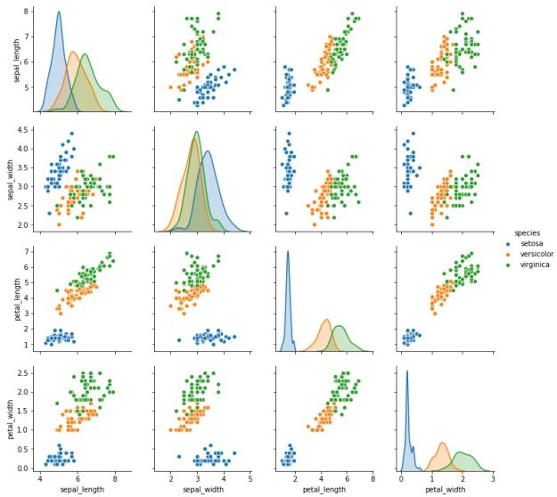
sns.pairplot(data=iris, hue="species")
【3】数据清洗
iris_simple = iris.drop(["sepal_length", "sepal_width"], axis=1)
iris_simple.head()
|
|
petal_length |
petal_width |
species |
| 0 |
1.4 |
0.2 |
setosa |
| 1 |
1.4 |
0.2 |
setosa |
| 2 |
1.3 |
0.2 |
setosa |
| 3 |
1.5 |
0.2 |
setosa |
| 4 |
1.4 |
0.2 |
setosa |
【4】标签编码
from sklearn.preprocessing import LabelEncoder
encoder = LabelEncoder()
iris_simple["species"] = encoder.fit_transform(iris_simple["species"])
iris_simple
|
|
petal_length |
petal_width |
species |
| 0 |
1.4 |
0.2 |
0 |
| 1 |
1.4 |
0.2 |
0 |
| ... |
... |
... |
... |
| 149 |
5.1 |
1.8 |
2 |
【5】数据集的标准化(本数据集特征比较接近,实际处理过程中未标准化)
from sklearn.preprocessing import StandardScaler
import pandas as pd
trans = StandardScaler()
_iris_simple = trans.fit_transform(iris_simple[["petal_length", "petal_width"]])
_iris_simple = pd.DataFrame(_iris_simple, columns = ["petal_length", "petal_width"])
_iris_simple.describe()
|
|
petal_length |
petal_width |
| count |
1.500000e+02 |
1.500000e+02 |
| mean |
-8.652338e-16 |
-4.662937e-16 |
| std |
1.003350e+00 |
1.003350e+00 |
| min |
-1.567576e+00 |
-1.447076e+00 |
| 25% |
-1.226552e+00 |
-1.183812e+00 |
| 50% |
3.364776e-01 |
1.325097e-01 |
| 75% |
7.627583e-01 |
7.906707e-01 |
| max |
1.785832e+00 |
1.712096e+00 |
【6】构建训练集和测试集(本课暂不考虑验证集)
from sklearn.model_selection import train_test_split
train_set, test_set = train_test_split(iris_simple, test_size=0.2)
test_set.head()
|
|
petal_length |
petal_width |
species |
| 3 |
1.5 |
0.2 |
0 |
| 111 |
5.3 |
1.9 |
2 |
| 24 |
1.9 |
0.2 |
0 |
| 5 |
1.7 |
0.4 |
0 |
| 92 |
4.0 |
1.2 |
1 |
iris_x_train = train_set[["petal_length", "petal_width"]]
iris_x_train.head()
|
|
petal_length |
petal_width |
| 63 |
4.7 |
1.4 |
| 93 |
3.3 |
1.0 |
| 34 |
1.5 |
0.2 |
| 35 |
1.2 |
0.2 |
| 126 |
4.8 |
1.8 |
iris_y_train = train_set["species"].copy()
iris_y_train.head()
63 1
93 1
34 0
35 0
126 2
Name: species, dtype: int32
iris_x_test = test_set[["petal_length", "petal_width"]]
iris_x_test.head()
|
|
petal_length |
petal_width |
| 3 |
1.5 |
0.2 |
| 111 |
5.3 |
1.9 |
| 24 |
1.9 |
0.2 |
| 5 |
1.7 |
0.4 |
| 92 |
4.0 |
1.2 |
iris_y_test = test_set["species"].copy()
iris_y_test.head()
3 0
111 2
24 0
5 0
92 1
Name: species, dtype: int32
14.2.k近邻算法
【1】基本思想
与待预测点最近的训练数据集中的k个邻居
把k个近邻中最常见的类别预测为带预测点的类别
【2】sklearn实现
from sklearn.neighbors import KNeighborsClassifier
构建分类器对象
clf = KNeighborsClassifier()
clf
KNeighborsClassifier(algorithm='auto', leaf_size=30, metric='minkowski',
metric_params=None, n_jobs=None, n_neighbors=5, p=2,
weights='uniform')
训练
clf.fit(iris_x_train, iris_y_train)
KNeighborsClassifier(algorithm='auto', leaf_size=30, metric='minkowski',
metric_params=None, n_jobs=None, n_neighbors=5, p=2,
weights='uniform')
预测
res = clf.predict(iris_x_test)
print(res)
print(iris_y_test.values)
[0 2 0 0 1 1 0 2 1 2 1 2 2 2 1 0 0 0 1 0 2 0 2 1 0 1 0 0 1 1]
[0 2 0 0 1 1 0 2 2 2 1 2 2 2 1 0 0 0 1 0 2 0 2 1 0 1 0 0 1 1]
翻转
encoder.inverse_transform(res)
array(['setosa', 'virginica', 'setosa', 'setosa', 'versicolor',
'versicolor', 'setosa', 'virginica', 'versicolor', 'virginica',
'versicolor', 'virginica', 'virginica', 'virginica', 'versicolor',
'setosa', 'setosa', 'setosa', 'versicolor', 'setosa', 'virginica',
'setosa', 'virginica', 'versicolor', 'setosa', 'versicolor',
'setosa', 'setosa', 'versicolor', 'versicolor'], dtype=object)
评估
accuracy = clf.score(iris_x_test, iris_y_test)
print("预测正确率:{:.0%}".format(accuracy))
预测正确率:97%
存储数据
out = iris_x_test.copy()
out["y"] = iris_y_test
out["pre"] = res
out
|
|
petal_length |
petal_width |
y |
pre |
| 3 |
1.5 |
0.2 |
0 |
0 |
| 111 |
5.3 |
1.9 |
2 |
2 |
| ... |
... |
... |
... |
... |
| 90 |
4.4 |
1.2 |
1 |
1 |
out.to_csv("iris_predict.csv")
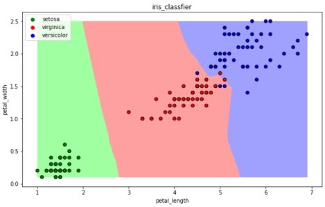
【3】可视化
import numpy as np
import matplotlib as mpl
import matplotlib.pyplot as plt
def draw(clf):
# 网格化
M, N = 500, 500
x1_min, x2_min = iris_simple[["petal_length", "petal_width"]].min(axis=0)
x1_max, x2_max = iris_simple[["petal_length", "petal_width"]].max(axis=0)
t1 = np.linspace(x1_min, x1_max, M)
t2 = np.linspace(x2_min, x2_max, N)
x1, x2 = np.meshgrid(t1, t2)
# 预测
x_show = np.stack((x1.flat, x2.flat), axis=1)
y_predict = clf.predict(x_show)
# 配色
cm_light = mpl.colors.ListedColormap(["#A0FFA0", "#FFA0A0", "#A0A0FF"])
cm_dark = mpl.colors.ListedColormap(["g", "r", "b"])
# 绘制预测区域图
plt.figure(figsize=(10, 6))
plt.pcolormesh(t1, t2, y_predict.reshape(x1.shape), cmap=cm_light)
# 绘制原始数据点
plt.scatter(iris_simple["petal_length"], iris_simple["petal_width"], label=None,
c=iris_simple["species"], cmap=cm_dark, marker='o', edgecolors='k')
plt.xlabel("petal_length")
plt.ylabel("petal_width")
# 绘制图例
color = ["g", "r", "b"]
species = ["setosa", "virginica", "versicolor"]
for i in range(3):
plt.scatter([], [], c=color[i], s=40, label=species[i]) # 利用空点绘制图例
plt.legend(loc="best")
plt.title('iris_classfier')
draw(clf)

14.3.朴素贝叶斯算法
【1】基本思想
当![]() 发生的时候,哪一个
发生的时候,哪一个![]() 发生的概率最大
发生的概率最大
【2】sklearn实现
from sklearn.naive_bayes import GaussianNB
构建分类器对象
clf = GaussianNB()
clf
训练
clf.fit(iris_x_train, iris_y_train)
预测
res = clf.predict(iris_x_test)
print(res)
print(iris_y_test.values)
[0 2 0 0 1 1 0 2 1 2 1 2 2 2 1 0 0 0 1 0 2 0 2 1 0 1 0 0 1 1]
[0 2 0 0 1 1 0 2 2 2 1 2 2 2 1 0 0 0 1 0 2 0 2 1 0 1 0 0 1 1]
评估
accuracy = clf.score(iris_x_test, iris_y_test)
print("预测正确率:{:.0%}".format(accuracy))
预测正确率:97%
可视化
draw(clf)
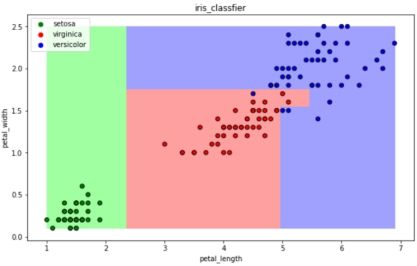
14.4.决策树算法
【1】基本思想
CART算法:每次通过一个特征,将数据尽可能的分为纯净的两类,递归的分下去
【2】sklearn实现
from sklearn.tree import DecisionTreeClassifier
构建分类器对象
clf = DecisionTreeClassifier()
clf
DecisionTreeClassifier(class_weight=None, criterion='gini', max_depth=None,
max_features=None, max_leaf_nodes=None,
min_impurity_decrease=0.0, min_impurity_split=None,
min_samples_leaf=1, min_samples_split=2,
min_weight_fraction_leaf=0.0, presort=False,
random_state=None, splitter='best')
训练
clf.fit(iris_x_train, iris_y_train)
预测
res = clf.predict(iris_x_test)
print(res)
print(iris_y_test.values)
[0 2 0 0 1 1 0 2 1 2 1 2 2 2 1 0 0 0 1 0 2 0 2 1 0 1 0 0 1 1]
[0 2 0 0 1 1 0 2 2 2 1 2 2 2 1 0 0 0 1 0 2 0 2 1 0 1 0 0 1 1]
评估
accuracy = clf.score(iris_x_test, iris_y_test)
print("预测正确率:{:.0%}".format(accuracy))
预测正确率:97%
可视化
draw(clf)
14.5.逻辑回归算法
【1】基本思想
一种解释:
训练:通过一个映射方式,将特征![]() 映射成
映射成 ![]() ,求使得所有概率之积最大化的映射方式里的参数
,求使得所有概率之积最大化的映射方式里的参数
预测:计算![]() 取概率最大的那个类别作为预测对象的分类
取概率最大的那个类别作为预测对象的分类
【2】sklearn实现
from sklearn.linear_model import LogisticRegression
构建分类器对象
clf = LogisticRegression(solver='saga', max_iter=1000)
clf
LogisticRegression(C=1.0, class_weight=None, dual=False, fit_intercept=True,
intercept_scaling=1, l1_ratio=None, max_iter=1000,
multi_class='warn', n_jobs=None, penalty='l2',
random_state=None, solver='saga', tol=0.0001, verbose=0,
warm_start=False)
训练
clf.fit(iris_x_train, iris_y_train)
预测
res = clf.predict(iris_x_test)
print(res)
print(iris_y_test.values)
[0 2 0 0 1 1 0 2 1 2 1 2 2 2 1 0 0 0 1 0 2 0 2 1 0 1 0 0 1 1]
[0 2 0 0 1 1 0 2 2 2 1 2 2 2 1 0 0 0 1 0 2 0 2 1 0 1 0 0 1 1]
评估
accuracy = clf.score(iris_x_test, iris_y_test)
print("预测正确率:{:.0%}".format(accuracy))
预测正确率:97%
可视化
draw(clf)

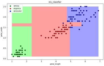
14.6.支持向量机算法
【1】基本思想
以二分类为例,假设数据可用完全分开:
用一个超平面将两类数据完全分开,且最近点到平面的距离最大
【2】sklearn实现
from sklearn.svm import SVC
构建分类器对象
clf = SVC()
clf
SVC(C=1.0, cache_size=200, class_weight=None, coef0=0.0,
decision_function_shape='ovr', degree=3, gamma='auto_deprecated',
kernel='rbf', max_iter=-1, probability=False, random_state=None,
shrinking=True, tol=0.001, verbose=False)
训练
clf.fit(iris_x_train, iris_y_train)
预测
res = clf.predict(iris_x_test)
print(res)
print(iris_y_test.values)
[0 2 0 0 1 1 0 2 1 2 1 2 2 2 1 0 0 0 1 0 2 0 2 1 0 1 0 0 1 1]
[0 2 0 0 1 1 0 2 2 2 1 2 2 2 1 0 0 0 1 0 2 0 2 1 0 1 0 0 1 1]
评估
accuracy = clf.score(iris_x_test, iris_y_test)
print("预测正确率:{:.0%}".format(accuracy))
预测正确率:97%
可视化
draw(clf)

14.7.集成方法——随机森林
【1】基本思想
训练集m,有放回的随机抽取m个数据,构成一组,共抽取n组采样集
n组采样集训练得到n个弱分类器 弱分类器一般用决策树或神经网络
将n个弱分类器进行组合得到强分类器
【2】sklearn实现
from sklearn.ensemble import RandomForestClassifier
构建分类器对象
clf = RandomForestClassifier()
clf
RandomForestClassifier(bootstrap=True, class_weight=None, criterion='gini',
max_depth=None, max_features='auto', max_leaf_nodes=None,
min_impurity_decrease=0.0, min_impurity_split=None,
min_samples_leaf=1, min_samples_split=2,
min_weight_fraction_leaf=0.0, n_estimators='warn',
n_jobs=None, oob_score=False, random_state=None,
verbose=0, warm_start=False)
训练
clf.fit(iris_x_train, iris_y_train)
预测
res = clf.predict(iris_x_test)
print(res)
print(iris_y_test.values)
[0 2 0 0 1 1 0 2 1 2 1 2 2 2 1 0 0 0 1 0 2 0 2 1 0 1 0 0 1 1]
[0 2 0 0 1 1 0 2 2 2 1 2 2 2 1 0 0 0 1 0 2 0 2 1 0 1 0 0 1 1]
评估
accuracy = clf.score(iris_x_test, iris_y_test)
print("预测正确率:{:.0%}".format(accuracy))
预测正确率:97%
可视化
draw(clf)

14.8.集成方法——Adaboost
【1】基本思想
训练集m,用初始数据权重训练得到第一个弱分类器,根据误差率计算弱分类器系数,更新数据的权重
使用新的权重训练得到第二个弱分类器,以此类推
根据各自系数,将所有弱分类器加权求和获得强分类器
【2】sklearn实现
from sklearn.ensemble import AdaBoostClassifier
构建分类器对象
clf = AdaBoostClassifier()
clf
AdaBoostClassifier(algorithm='SAMME.R', base_estimator=None, learning_rate=1.0,
n_estimators=50, random_state=None)
训练
clf.fit(iris_x_train, iris_y_train)
预测
res = clf.predict(iris_x_test)
print(res)
print(iris_y_test.values)
[0 2 0 0 1 1 0 2 1 2 1 2 2 2 1 0 0 0 1 0 2 0 2 1 0 1 0 0 1 1]
[0 2 0 0 1 1 0 2 2 2 1 2 2 2 1 0 0 0 1 0 2 0 2 1 0 1 0 0 1 1]
评估
accuracy = clf.score(iris_x_test, iris_y_test)
print("预测正确率:{:.0%}".format(accuracy))
预测正确率:97%
可视化
draw(clf)

14.9.集成方法——梯度提升树GBDT
【1】基本思想
训练集m,获得第一个弱分类器,获得残差,然后不断地拟合残差
所有弱分类器相加得到强分类器
【2】sklearn实现
from sklearn.ensemble import GradientBoostingClassifier
构建分类器对象
clf = GradientBoostingClassifier()
clf
GradientBoostingClassifier(criterion='friedman_mse', init=None,
learning_rate=0.1, loss='deviance', max_depth=3,
max_features=None, max_leaf_nodes=None,
min_impurity_decrease=0.0, min_impurity_split=None,
min_samples_leaf=1, min_samples_split=2,
min_weight_fraction_leaf=0.0, n_estimators=100,
n_iter_no_change=None, presort='auto',
random_state=None, subsample=1.0, tol=0.0001,
validation_fraction=0.1, verbose=0,
warm_start=False)
训练
clf.fit(iris_x_train, iris_y_train)
预测
res = clf.predict(iris_x_test)
print(res)
print(iris_y_test.values)
[0 2 0 0 1 1 0 2 1 2 1 2 2 2 1 0 0 0 1 0 2 0 2 1 0 1 0 0 1 1]
[0 2 0 0 1 1 0 2 2 2 1 2 2 2 1 0 0 0 1 0 2 0 2 1 0 1 0 0 1 1]
评估
accuracy = clf.score(iris_x_test, iris_y_test)
print("预测正确率:{:.0%}".format(accuracy))
预测正确率:97%
可视化
draw(clf)
14.10.扩展
【1】xgboost
GBDT的损失函数只对误差部分做负梯度(一阶泰勒)展开
XGBoost损失函数对误差部分做二阶泰勒展开,更加准确,更快收敛
【2】lightgbm
微软:快速的,分布式的,高性能的基于决策树算法的梯度提升框架
速度更快
【3】stacking
堆叠或者叫模型融合
先建立几个简单的模型进行训练,第二级学习器会基于前级模型的预测结果进行再训练
【4】神经网络