【cs224n学习作业】Assignment 1 - Exploring Word Vectors【附代码】

前言

这篇文章是CS224N课程的第一个大作业， 主要是对词向量做了一个探索， 并直观的感受了一下词嵌入或者词向量的效果。这里简单的记录一下我探索的一个过程。 这一下几篇文章基于这次作业的笔记理论：
cs224n学习笔记 01: Introduction and word vectors.
cs224n学习笔记 02:Word Vectors and Word Senses.
cs224n学习笔记 03:Subword Models（fasttext附代码）.
cs224n学习笔记 04：Contextual Word Embeddings.
此次实验分为两部分， 第一部分是基于计数的单词词向量， 而第二部分，是基于词向量的预测， 是利用了已经训练好的一个词向量矩阵去介绍一下怎么进行预测， 比如可视化这些词向量啊， 找同义词或者反义词啊，实现单词的类比关系啊等等。

大纲

• 实验前的准备工作(导入包和语料库)
• Part1: Count-Based Word Vectors
• Part2:Prediction-Based Word Vectors

准备工作

导入要用的包

import sys
assert sys.version_info[0]==3
assert sys.version_info[1] >= 5

from gensim.models import KeyedVectors  # KeyedVectors:实现实体（单词、文档、图片都可以）和向量之间的映射。每个实体由其字符串id标识。
from gensim.test.utils import datapath
import pprint     #  输出的更加规范易读
import matplotlib.pyplot as plt  
plt.rcParams['figure.figsize'] = [10, 5]  #  plt.rcParams主要作用是设置画的图的分辨率，大小等信息
import nltk
nltk.download('reuters')    # 这个可以从GitHub下载， 网址：https://github.com/nltk/nltk_data/tree/gh-pages/packages/corpora
from nltk.corpus import reuters
import numpy as np
import random
import scipy as sp
from sklearn.decomposition import TruncatedSVD
from sklearn.decomposition import PCA

START_TOKEN = ''
END_TOKEN = ''

np.random.seed(0)
random.seed(0)

这里面的Reuters是路透社(商业和金融新闻)语料库， 是一个词库， 语料库包含10788个新闻文档，共计130万词。这些文档跨越90个类别，分为train和test，我们这次需要用其中的一个类别(crude)里面的句子。
对于这个数据集以及后面要用到的数据我们直接下下不来，所以这里提供另外一个方法就是自己可以百度手动下载数据集。这些数据网上都有都是可以自行下载过来的。
然后就是采用下面的函数，导入这个语料库：

def read_corpus(category="crude"):
    """ Read files from the specified Reuter's category.
        Params:
            category (string): category name
        Return:
            list of lists, with words from each of the processed files
    """
    files = reuters.fileids(category)    # 类别为crude文档
    # 每个文档都转化为小写， 并在开头结尾加标识符
    return [[START_TOKEN] + [w.lower() for w in list(reuters.words(f))] + [END_TOKEN] for f in files]

这个是导入语料库的函数， 简单的进行了一下预处理， 就是在每句话的前面和后面各加了一个标识符，表示句子的开始和结束，然后把每个单词分开。 下面导入并看一下效果：

# pprint模块格式化打印
# pprint.pprint(object, stream=None, indent=1, width=80, depth=None, *, compact=False)
# width：控制打印显示的宽度。默认为80个字符。注意：当单个对象的长度超过width时，并不会分多行显示，而是会突破规定的宽度。
# compact：默认为False。如果值为False，超过width规定长度的序列会被分散打印到多行。如果为True，会尽量使序列填满width规定的宽度。
reuters_corpus = read_corpus()
pprint.pprint(reuters_corpus[:1], compact=True, width=100)  # compact 设置为False是一行一个单词

每个句子处理后长这样：

准备工作完成，接下来就是实验的主要两部分了。

Part1: Count-Based Word Vectors

共现矩阵是实现这种词向量的一种方式， 我们看看共现矩阵是什么意思？ 共现矩阵计算的是单词在某些环境下一块出现的频率， 对于共现矩阵， 原文描述是这样的：

上面的话其实就是这样的一个意思， 要想建立共现矩阵，我们需要先为单词构建一个词典， 然后共现矩阵的行列都是这个词典里的单词， 看下面这个例子：

上面基于这两段文档构建出的共现矩阵长这样， 这个是怎么构建的？ 首先就是根据两个文档的单词构建一个词典， 这里面的数就是两两单词在上下文中共现的频率， 比如第一行， START和all一起出现了两次， 这就是因为两个文档里面START的窗口中都有all。 同理第二行all的那个， 我们也固定一个窗口， 发现第一个文档里面all左边是START， 右边是that， 第二个文档all左边是START， 右边是is, 那么=2, =1, =1。 下面的都是同理了。

我们就是要构建这样的一个矩阵来作为每个单词的词向量， 当然这个还不是最终形式， 因为可能词典很大的话维度会特别高， 所以就相当了降维技术， 降维之后的结果就是每个单词的词向量。 这个里面使用的降维是SVD, 原理这里不说， 这里使用了Truncated SVD， 具体的实现是调用了sklearn中的包。

所以我们就有了下面的这样一个思路框架：

1. 对于语录料库中的文档单词， 得先构建一个词典（唯一单词且排好序）
2. 然后我们就是基于词典和语料库，为每个单词构建词向量， 也就是共现矩阵
3. 对共现矩阵降维，就得到了最终的词向量
4. 可视化

1.1为语料库中的单词构建词典

词典就是记录所有的单词， 但是单词唯一且有序。 那么实现这个词典的思路就是我遍历每一篇文档，先获得所有的单词， 然后去掉重复的， 然后再排序就搞定， 当然还得记录字典里的单词总数。

# 计算出语料库中出现的不同单词，并排序。
def distinct_words(corpus):
    """ Determine a list of distinct words for the corpus.
        Params:
            corpus (list of list of strings): corpus of documents
        Return:
            corpus_words (list of strings): list of distinct words across the corpus, sorted (using python 'sorted' function)
            num_corpus_words (integer): number of distinct words across the corpus
    """
    corpus_words = []
    num_corpus_words = -1
    
    # ------------------
    # Write your implementation here.
    # 首先得把所有单词放到一个列表里面, 然后用set去重， 然后排序
    for everylist in corpus:
        corpus_words.extend(everylist)
    corpus_words = sorted(set(corpus_words))
    num_corpus_words = len(corpus_words)
    # ------------------

    return corpus_words, num_corpus_words

1.2 构建共现矩阵

首先我们得定义一个M矩阵， 也就是共现矩阵， 大小就是行列都是词典的单词个数（上面图片一目了然）， 然后还得定义一个字典单词到索引的映射， 因为我们统计的时候是遍历真实文档， 而填矩阵的时候是基于字典，这两个是基于同一个单词进行联系起来的， 所以我们需要获得真实文档中单词在字典里面的索引才能去填矩阵。

def compute_co_occurrence_matrix(corpus, window_size=4):
    """ Compute co-occurrence matrix for the given corpus and window_size (default of 4).
    
        Note: Each word in a document should be at the center of a window. Words near edges will have a smaller
              number of co-occurring words.
              
              For example, if we take the document "START All that glitters is not gold END" with window size of 4,
              "All" will co-occur with "START", "that", "glitters", "is", and "not".
    
        Params:
            corpus (list of list of strings): corpus of documents
            window_size (int): size of context window
        Return:
            M (numpy matrix of shape (number of corpus words, number of corpus words)): 
                Co-occurence matrix of word counts. 
                The ordering of the words in the rows/columns should be the same as the ordering of the words given by the distinct_words function.
            word2Ind (dict): dictionary that maps word to index (i.e. row/column number) for matrix M.
    """
    words, num_words = distinct_words(corpus)   # 单词已经去重或者排好序  
    M = None
    word2Ind = {}
    
    # ------------------
    # Write your implementation here.
    word2Ind = {k: v for (k, v) in zip(words, range(num_words))}
    M = np.zeros((num_words, num_words))
    	# 接下来是遍历语料库 对于每一篇文档， 我们得遍历每个单词
    # 对于每个单词， 我们得找到窗口的范围， 然后再去遍历它窗口内的每个单词
    # 对于这每个单词， 我们就可以在我们的M词典中进行计数， 但是要注意每个单词其实有两个索引
    # 一个是词典里面的索引， 一个是文档中的索引， 我们统计的共现频率是基于字典里面的索引， 
    # 所以这里涉及到一个索引的转换
    
    # 首先遍历语料库
    for every_doc in corpus:
        for cword_doc_ind, cword in enumerate(every_doc):  # 遍历当前文档的每个单词和在文档中的索引
            # 对于当前的单词， 我们先找到它在词典中的位置
            cword_dic_ind = word2Ind[cword]
            
            # 找窗口的起始和终止位置  开始位置就是当前单词的索引减去window_size, 终止位置
            # 是当前索引加上windo_size+1， 
            window_start = cword_doc_ind - window_size
            window_end = cword_doc_ind + window_size + 1
            
            # 有了窗口， 我们就要遍历窗口里面的每个单词， 然后往M里面记录就行了
            # 但是还要注意一点， 就是边界问题， 因为开始单词左边肯定不够窗口大小， 结束单词
            # 右边肯定不够窗口大小， 所以遍历之后得判断一下是不是左边后者右边有单词
            for j in range(window_start, window_end):
                # 前面两个条件控制不越界， 最后一个条件控制不是它本身
                if j >=0 and j < len(every_doc) and j != cword_doc_ind:
                    # 想办法加入到M， 那么得获取这个单词在词典中的位置
                    oword = every_doc[j]   # 获取到上下文单词
                    oword_dic_ind = word2Ind[oword]
                    # 加入M
                    M[cword_dic_ind, oword_dic_ind] += 1
    # ------------------

    return M, word2Ind

3.3 降维到K维

降维直接调用包SVD.

def reduce_to_k_dim(M, k=2):
    """ Reduce a co-occurence count matrix of dimensionality (num_corpus_words, num_corpus_words)
        to a matrix of dimensionality (num_corpus_words, k) using the following SVD function from Scikit-Learn:
            - http://scikit-learn.org/stable/modules/generated/sklearn.decomposition.TruncatedSVD.html
    
        Params:
            M (numpy matrix of shape (number of corpus words, number of corpus words)): co-occurence matrix of word counts
            k (int): embedding size of each word after dimension reduction
        Return:
            M_reduced (numpy matrix of shape (number of corpus words, k)): matrix of k-dimensioal word embeddings.
                    In terms of the SVD from math class, this actually returns U * S
    """    
    n_iters = 10     # Use this parameter in your call to `TruncatedSVD`
    M_reduced = None
    print("Running Truncated SVD over %i words..." % (M.shape[0]))
    
        # ------------------
        # Write your implementation here.
    svd = TruncatedSVD(n_components=k, n_iter=n_iters, random_state=2020)
    M_reduced = svd.fit_transform(M)
        # ------------------

    print("Done.")
    return M_reduced

最后可视化结果

def plot_embeddings(M_reduced, word2Ind, words):
    """ Plot in a scatterplot the embeddings of the words specified in the list "words".
        NOTE: do not plot all the words listed in M_reduced / word2Ind.
        Include a label next to each point.
        
        Params:
            M_reduced (numpy matrix of shape (number of unique words in the corpus , k)): matrix of k-dimensioal word embeddings
            word2Ind (dict): dictionary that maps word to indices for matrix M
            words (list of strings): words whose embeddings we want to visualize
    """

    # ------------------
    # Write your implementation here.
    # 遍历句子， 获得每个单词的x，y坐标
    for word in words:
        word_dic_index = word2Ind[word]
        x = M_reduced[word_dic_index][0]
        y = M_reduced[word_dic_index][1]
        plt.scatter(x, y, marker='x', color='red')
        # plt.text()给图形添加文本注释
        plt.text(x+0.0002, y+0.0002, word, fontsize=9)  # # x、y上方0.002处标注文字说明，word标注的文字，fontsize：文字大小
    plt.show()
    # ------------------

综合以上的步骤：首先是读入数据， 然后计算共现矩阵， 然后是降维， 最后是可视化：

reuters_corpus = read_corpus()
M_co_occurrence, word2Ind_co_occurrence = compute_co_occurrence_matrix(reuters_corpus)
M_reduced_co_occurrence = reduce_to_k_dim(M_co_occurrence, k=2)

# Rescale (normalize) the rows to make them each of unit-length
M_lengths = np.linalg.norm(M_reduced_co_occurrence, axis=1)
M_normalized = M_reduced_co_occurrence / M_lengths[:, np.newaxis] # broadcasting

words = ['barrels', 'bpd', 'ecuador', 'energy', 'industry', 'kuwait', 'oil', 'output', 'petroleum', 'venezuela']
plot_embeddings(M_normalized, word2Ind_co_occurrence, words)

得到结果如下：

Part2:Prediction-Based Word Vectors

2.1 可视化Word2Vec训练的词嵌入

这一部分其实是利用了一个用Word2Vec技术训练好的词向量矩阵去测试一些有趣的效果， 看看词向量到底是干啥用的。 所以用gensim包下载了一个词向量矩阵：

def load_word2vec(embeddings_fp="F:\\jupyter lab./GoogleNews-vectors-negative300.bin"):
    """ Load Word2Vec Vectors
        Param:
            embeddings_fp (string) - path to .bin file of pretrained word vectors
        Return:
            wv_from_bin: All 3 million embeddings, each lengh 300
                This is the KeyedVectors format: https://radimrehurek.com/gensim/models/deprecated/keyedvectors.html
    """
    embed_size = 300
    print("Loading 3 million word vectors from file...")
    ## 自己下载的文件
    wv_from_bin = KeyedVectors.load_word2vec_format(embeddings_fp, binary=True)
    vocab = list(wv_from_bin.vocab.keys())
    print("Loaded vocab size %i" % len(vocab))
    return wv_from_bin
wv_from_bin = load_word2vec()

路径换成自己的数据保存路径就行

有了这个代码，我们就能得到一个基于Word2Vec训练好的词向量矩阵（和上面我们的M矩阵是类似的，只不过得到的方式不同）， 接下来就是进行降维并可视化词嵌入：

def get_matrix_of_vectors(wv_from_bin, required_words=['barrels', 'bpd', 'ecuador', 'energy', 'industry', 'kuwait', 'oil', 'output', 'petroleum', 'venezuela']):
    """ Put the word2vec vectors into a matrix M.
        Param:
            wv_from_bin: KeyedVectors object; the 3 million word2vec vectors loaded from file
        Return:
            M: numpy matrix shape (num words, 300) containing the vectors
            word2Ind: dictionary mapping each word to its row number in M
    """
    import random
    words = list(wv_from_bin.vocab.keys())
    print("Shuffling words ...")
    random.shuffle(words)
    words = words[:10000]       # 选10000个加入
    print("Putting %i words into word2Ind and matrix M..." % len(words))
    word2Ind = {}
    M = []
    curInd = 0
    for w in words:
        try:
            M.append(wv_from_bin.word_vec(w))
            word2Ind[w] = curInd
            curInd += 1
        except KeyError:
            continue
    for w in required_words:
        try:
            M.append(wv_from_bin.word_vec(w))
            word2Ind[w] = curInd
            curInd += 1
        except KeyError:
            continue
    M = np.stack(M)
    print("Done.")
    return M, word2Ind

# -----------------------------------------------------------------
# Run Cell to Reduce 300-Dimensinal Word Embeddings to k Dimensions
# Note: This may take several minutes
# -----------------------------------------------------------------
M, word2Ind = get_matrix_of_vectors(wv_from_bin)
M_reduced = reduce_to_k_dim(M, k=2)         # 减到了2维

words = ['barrels', 'bpd', 'ecuador', 'energy', 'industry', 'kuwait', 'oil', 'output', 'petroleum', 'venezuela']
plot_embeddings(M_reduced, word2Ind, words)

结果如下：

2.2 余弦相似度

我们已经得到了每个单词的词向量表示， 那么怎么看两个单词的相似性程度呢？ 余弦相似性是一种方式， 公式如下：

基于这个方式，我们就可以找到单词的多义词， 同义词，反义词还能实现单词的类比推理等。所以是直接调用的gensim的函数就行。

# 找和energy最相近的10个单词
wv_from_bin.most_similar("energy")

##结果
[('renewable_energy', 0.6721636056900024),
 ('enery', 0.6289607286453247),
 ('electricity', 0.6030439138412476),
 ('enegy', 0.6001754403114319),
 ('Energy', 0.595537006855011),
 ('fossil_fuel', 0.5802257061004639),
 ('natural_gas', 0.5767925381660461),
 ('renewables', 0.5708995461463928),
 ('fossil_fuels', 0.5689164996147156),
 ('renewable', 0.5663810968399048)]

再比如， 为我们可以找同义词和反义词：

w1 = "man"
w2 = "king"
w3 = "woman"
w1_w2_dist = wv_from_bin.distance(w1, w2)
w1_w3_dist = wv_from_bin.distance(w1, w3)

print("Synonyms {}, {} have cosine distance: {}".format(w1, w2, w1_w2_dist))
print("Antonyms {}, {} have cosine distance: {}".format(w1, w3, w1_w3_dist))

## 结果：
Synonyms man, king have cosine distance: 0.7705732733011246
Antonyms man, woman have cosine distance: 0.2335987687110901

还可以实现类比关系：
比如： China : Beijing = Japan : ?， 那么我们可以用下面的代码求这样的类别关系， 注意下面的positive和negative里面的单词顺序， 我们求得？其实和Japan和Beijing相似， 和China远。

# Run this cell to answer the analogy -- man : king :: woman : x
pprint.pprint(wv_from_bin.most_similar(positive=['Bejing', 'Japan'], negative=['China']))

## 结果：
[('Tokyo', 0.6124968528747559),
 ('Osaka', 0.5791803598403931),
 ('Maebashi', 0.5635818243026733),
 ('Fukuoka_Japan', 0.5362966060638428),
 ('Nagoya', 0.5359445214271545),
 ('Fukuoka', 0.5319067239761353),
 ('Osaka_Japan', 0.5298740267753601),
 ('Nagano', 0.5293833017349243),
 ('Taisuke', 0.5258569717407227),
 ('Chukyo', 0.5195443034172058)]

2.3 引导词向量偏差分析

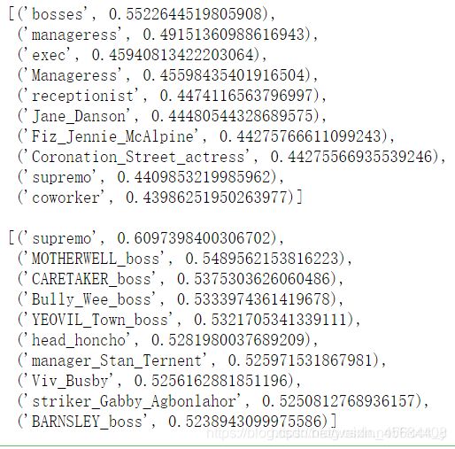
识别单词嵌入隐含的偏见(性别、种族、性取向等)。
运行下面的单元格，检查
(a)哪些词与“woman”和“boss”最相似，而与“man”最不相似;
(b)哪些词与“man”和“boss”最相似，而与“woman”最不相似。

# Run this cell
# Here `positive` indicates the list of words to be similar to and `negative` indicates the list of words to be
# most dissimilar from.
#这里“positive”表示类似的单词列表，而“negative”表示是最不相似于。
pprint.pprint(wv_from_bin.most_similar(positive=['woman', 'boss'], negative=['man']))
print()
pprint.pprint(wv_from_bin.most_similar(positive=['man', 'boss'], negative=['woman']))

得到结果如下：

2.4 独立的单词向量偏差分析

# ------------------
# Write your bias exploration code here.

pprint.pprint(wv_from_bin.most_similar(positive=['woman', 'doctor'], negative=['man']))
print()
pprint.pprint(wv_from_bin.most_similar(positive=['woman', 'nurse'], negative=['man']))

# ------------------

结果如下：

【附完整代码】

# 导入包
import sys
assert sys.version_info[0]==3
assert sys.version_info[1] >= 5

from gensim.models import KeyedVectors  # KeyedVectors:实现实体（单词、文档、图片都可以）和向量之间的映射。每个实体由其字符串id标识。
from gensim.test.utils import datapath
import pprint     #  输出的更加规范易读
import matplotlib.pyplot as plt
plt.rcParams['figure.figsize'] = [10, 5]  #  plt.rcParams主要作用是设置画的图的分辨率，大小等信息
# import nltk
# nltk.download('reuters')    # 这个可以从GitHub下载， 网址：https://github.com/nltk/nltk_data/tree/gh-pages/packages/corpora
from nltk.corpus import reuters
import numpy as np
import random
import rando
import scipy as sp
from sklearn.decomposition import TruncatedSVD
from sklearn.decomposition import PCA

START_TOKEN = ''
END_TOKEN = ''

np.random.seed(0)
random.seed(0)

# 导入 "reuters" 语料库
def read_corpus(category="crude"):
    """ Read files from the specified Reuter's category.
        Params:
            category (string): category name
        Return:
            list of lists, with words from each of the processed files
    """
    files = reuters.fileids(category)    # 类别为crude文档
    # 每个文档都转化为小写， 并在开头结尾加标识符
    return [[START_TOKEN] + [w.lower() for w in list(reuters.words(f))] + [END_TOKEN] for f in files]
print()

# 导入语料库的函数，简单的进行了一下预处理，
# 在每句话的前面和后面各加了一个标识符，表示句子的开始和结束，然后把每个单词分开。
# pprint模块格式化打印
# pprint.pprint(object, stream=None, indent=1, width=80, depth=None, *, compact=False)
# width：控制打印显示的宽度。默认为80个字符。注意：当单个对象的长度超过width时，并不会分多行显示，而是会突破规定的宽度。
# compact：默认为False。如果值为False，超过width规定长度的序列会被分散打印到多行。如果为True，会尽量使序列填满width规定的宽度。
reuters_corpus = read_corpus()
pprint.pprint(reuters_corpus[:1], compact=True, width=100)  # compact 设置为False是一行一个单词

# 问题1.1：实现不同单词
# 计算语料库的单词数量、单词集
def distinct_words(corpus):
    """ Determine a list of distinct words for the corpus.
        Params:
            corpus (list of list of strings): corpus of documents
        Return:
            corpus_words (list of strings): list of distinct words across the corpus, sorted (using python 'sorted' function)
            num_corpus_words (integer): number of distinct words across the corpus
    """
    corpus_words = []
    num_corpus_words = -1

    # Write your implementation here.
    corpus = [w for sent in corpus for w in sent]
    corpus_words = list(set(corpus))
    corpus_words = sorted(corpus_words)
    num_corpus_words = len(corpus_words)
    # 返回的结果是语料库中的所有单词按照字母顺序排列的。
    return corpus_words, num_corpus_words

# 问题1.2：实现共现矩阵
# 计算给定语料库的共现矩阵。具体来说，对于每一个词 w，统计前、后方 window_size 个词的出现次数\
def compute_co_occurrence_matrix(corpus, window_size=4):
    """ Compute co-occurrence matrix for the given corpus and window_size (default of 4).

        Note: Each word in a document should be at the center of a window. Words near edges will have a smaller
              number of co-occurring words.

              For example, if we take the document "START All that glitters is not gold END" with window size of 4,
              "All" will co-occur with "START", "that", "glitters", "is", and "not".

        Params:
            corpus (list of list of strings): corpus of documents
            window_size (int): size of context window
        Return:
            M (numpy matrix of shape (number of corpus words, number of corpus words)):
                Co-occurence matrix of word counts.
                The ordering of the words in the rows/columns should be the same as the ordering of the words given by the distinct_words function.
            word2Ind (dict): dictionary that maps word to index (i.e. row/column number) for matrix M.
    """
    words, num_words = distinct_words(corpus)
    M = None
    word2Ind = {}

    # Write your implementation here.
    M = np.zeros(shape=(num_words, num_words), dtype=np.int32)
    for i in range(num_words):
        word2Ind[words[i]] = i

    for sent in corpus:
        for p in range(len(sent)):
            ci = word2Ind[sent[p]]

            # preceding
            for w in sent[max(0, p - window_size):p]:
                wi = word2Ind[w]
                M[ci][wi] += 1

            # subsequent
            for w in sent[p + 1:p + 1 + window_size]:
                wi = word2Ind[w]
                M[ci][wi] += 1

    return M, word2Ind

# 问题1.3：实现降到k维
# 这一步是降维。
# 在问题1.2得到的是一个N x N的矩阵（N是单词集的大小），使用scikit-learn实现的SVD（奇异值分解），从这个大矩阵里分解出一个含k个特制的N x k 小矩阵。
def reduce_to_k_dim(M, k=2):
    """ Reduce a co-occurence count matrix of dimensionality (num_corpus_words, num_corpus_words)
        to a matrix of dimensionality (num_corpus_words, k) using the following SVD function from Scikit-Learn:
            - http://scikit-learn.org/stable/modules/generated/sklearn.decomposition.TruncatedSVD.html

        Params:
            M (numpy matrix of shape (number of corpus words, number of corpus words)): co-occurence matrix of word counts
            k (int): embedding size of each word after dimension reduction
        Return:
            M_reduced (numpy matrix of shape (number of corpus words, k)): matrix of k-dimensioal word embeddings.
                    In terms of the SVD from math class, this actually returns U * S
    """
    n_iters = 10  # Use this parameter in your call to `TruncatedSVD`
    M_reduced = None
    print("Running Truncated SVD over %i words..." % (M.shape[0]))

    # Write your implementation here.
    svd = TruncatedSVD(n_components=k)
    svd.fit(M.T)
    M_reduced = svd.components_.T

    print("Done.")
    return M_reduced

# 问题1.4 实现 plot_embeddings
# 编写一个函数来绘制2D空间中的一组2D矢量。
# 基于matplotlib，用scatter 画 “×”，用 text 写字
def plot_embeddings(M_reduced, word2Ind, words):
    """ Plot in a scatterplot the embeddings of the words specified in the list "words".
        NOTE: do not plot all the words listed in M_reduced / word2Ind.
        Include a label next to each point.

        Params:
            M_reduced (numpy matrix of shape (number of unique words in the corpus , 2)): matrix of 2-dimensioal word embeddings
            word2Ind (dict): dictionary that maps word to indices for matrix M
            words (list of strings): words whose embeddings we want to visualize
    """
    # Write your implementation here.
    fig = plt.figure()
    plt.style.use("seaborn-whitegrid")
    for word in words:
        point = M_reduced[word2Ind[word]]
        plt.scatter(point[0], point[1], marker="^")
        plt.annotate(word, xy=(point[0], point[1]), xytext=(point[0], point[1] + 0.1))

# 测试解决方案图
print("-" * 80)
print("Outputted Plot:")

M_reduced_plot_test = np.array([[1, 1], [-1, -1], [1, -1], [-1, 1], [0, 0]])
word2Ind_plot_test = {'test1': 0, 'test2': 1, 'test3': 2, 'test4': 3, 'test5': 4}
words = ['test1', 'test2', 'test3', 'test4', 'test5']
plot_embeddings(M_reduced_plot_test, word2Ind_plot_test, words)

print("-" * 80)
print()

# 问题1.5：共现打印分析
# 将词嵌入到2个维度上，归一化，最终词向量会落到一个单位圆内，在坐标系上寻找相近的词。
reuters_corpus = read_corpus()
M_co_occurrence, word2Ind_co_occurrence = compute_co_occurrence_matrix(reuters_corpus)
M_reduced_co_occurrence = reduce_to_k_dim(M_co_occurrence, k=2)

# Rescale (normalize) the rows to make them each of unit-length
M_lengths = np.linalg.norm(M_reduced_co_occurrence, axis=1)
M_normalized = M_reduced_co_occurrence / M_lengths[:, np.newaxis] # broadcasting

words = ['barrels', 'bpd', 'ecuador', 'energy', 'industry', 'kuwait', 'oil', 'output', 'petroleum', 'venezuela']

plot_embeddings(M_normalized, word2Ind_co_occurrence, words)
plt.show()

# Part 2：基于预测的词向量
# 使用gensim探索词向量，不是自己实现word2vec，所使用的词向量维度是300，由google发布。
def load_word2vec(embeddings_fp="./GoogleNews-vectors-negative300.bin"):
    """ Load Word2Vec Vectors
        Param:
            embeddings_fp (string) - path to .bin file of pretrained word vectors
        Return:
            wv_from_bin: All 3 million embeddings, each lengh 300
                This is the KeyedVectors format: https://radimrehurek.com/gensim/models/deprecated/keyedvectors.html
    """
    embed_size = 300
    print("Loading 3 million word vectors from file...")
    ## 自己下载的文件
    wv_from_bin = KeyedVectors.load_word2vec_format(embeddings_fp, binary=True)
    vocab = list(wv_from_bin.vocab.keys())
    print("Loaded vocab size %i" % len(vocab))
    return wv_from_bin
wv_from_bin = load_word2vec()
print()

# 首先使用SVD降维，将300维降2维，方便打印查看。
# 问题2.1：word2vec打印分析
# 和问题1.5一样
def get_matrix_of_vectors(wv_from_bin, required_words=['barrels', 'bpd', 'ecuador', 'energy', 'industry', 'kuwait', 'oil', 'output', 'petroleum', 'venezuela']):
    """ Put the word2vec vectors into a matrix M.
        Param:
            wv_from_bin: KeyedVectors object; the 3 million word2vec vectors loaded from file
        Return:
            M: numpy matrix shape (num words, 300) containing the vectors
            word2Ind: dictionary mapping each word to its row number in M
    """
    import random
    words = list(wv_from_bin.vocab.keys())
    print("Shuffling words ...")
    random.shuffle(words)
    words = words[:10000]       # 选10000个加入
    print("Putting %i words into word2Ind and matrix M..." % len(words))
    word2Ind = {}
    M = []
    curInd = 0
    for w in words:
        try:
            M.append(wv_from_bin.word_vec(w))
            word2Ind[w] = curInd
            curInd += 1
        except KeyError:
            continue
    for w in required_words:
        try:
            M.append(wv_from_bin.word_vec(w))
            word2Ind[w] = curInd
            curInd += 1
        except KeyError:
            continue
    M = np.stack(M)
    print("Done.")
    return M, word2Ind

# 测试解决方案图
print("-" * 80)
print("Outputted Plot:")
print("-" * 80)

M, word2Ind = get_matrix_of_vectors(wv_from_bin)
M_reduced = reduce_to_k_dim(M, k=2)         # 减到了2维
plt.tight_layout()
words = ['barrels', 'bpd', 'ecuador', 'energy', 'industry', 'kuwait', 'oil', 'output', 'petroleum', 'venezuela']
plot_embeddings(M_reduced, word2Ind, words)
plt.show()

# 问题2.2：一词多义
# 找到一个有多个含义的词（比如 “leaves”，“scoop”），这种词的top-10相似词（根据余弦相似度）里有两个词的意思不一样。比如"leaves"（叶子，花瓣）的top-10词里有"vanishes"（消失）和"stalks"（茎秆）。
# 这里我找到的词是"column"（列），它的top-10里有"columnist"（专栏作家）和"article"（文章）
w0 = "column"
w0_mean = wv_from_bin.most_similar(w0)
print("column：", w0_mean)
print()

# 问题2.3：近义词和反义词
# 找到三个词(w1, w2, w3)，其中w1和w2是近义词，w1和w3是反义词，但是w1和w3的距离
# 例如：w1=“happy”，w2=“cheerful”，w3=“sad”
w1 = "love"
w2 = "like"
w3 = "hate"
w1_w2_dist = wv_from_bin.distance(w1, w2)
w1_w3_dist = wv_from_bin.distance(w1, w3)
print("Synonyms {}, {} have cosine distance: {}".format(w1, w2, w1_w2_dist))
print("Antonyms {}, {} have cosine distance: {}".format(w1, w3, w1_w3_dist))
print()

# 问题2.4：类比
# man 对于 king，相当于woman对于___，这样的问题也可以用word2vec来解决
# man : him :: woman : her
print("类比 man : him :: woman : her：")
pprint.pprint(wv_from_bin.most_similar(positive=['woman', 'him'], negative=['man']))
print()


# 问题2.5：错误的类比
# 找到一个错误的类比，树：树叶 ：：花：花瓣
print("错误的类比 tree : leaf :: flower : petal：")
pprint.pprint(wv_from_bin.most_similar(positive=['leaf', 'flower'], negative=['tree']))
print()

# 问题2.6：偏见分析
# 注意偏见是很重要的比如性别歧视、种族歧视等，执行下面代码，分析两个问题：
# (a) 哪个词与“woman”和“boss”最相似，和“man”最不相似?
# (b) 哪个词与“man”和“boss”最相似，和“woman”最不相似?
print("偏见 woman : boss :: man：")
pprint.pprint(wv_from_bin.most_similar(positive=['woman', 'boss'], negative=['man']))
print()
print("偏见 man : boss :: woman：")
pprint.pprint(wv_from_bin.most_similar(positive=['man', 'boss'], negative=['woman']))
print()

# 问题2.7：自行分析偏见
#     男人:女人 :: 医生:___
#     女人:男人 :: 医生:___
print("自行分析偏见 woman : doctor :: man：")
pprint.pprint(wv_from_bin.most_similar(positive=['woman', 'doctor'], negative=['man']))
print()
print("自行分析偏见 man : doctor :: woman：")
pprint.pprint(wv_from_bin.most_similar(positive=['man', 'doctor'], negative=['woman']))
print()