第三章 Python Pandas数据分析运用

三、Python Pandas数据分析运用

1. Pandas常用数据结构

创建一个series对象

• series1 = pd.Series([2.8,3.01,8.99,8.59,5.18]) #序列
• series2 = pd.Series([2.8,3.01,8.99,8.59,5.18], index = [‘a’,‘b’,‘c’,‘d’,‘e’],name=‘This is a series’)
  #index：索引
• series6 = series4.append(series5) #增加
• series6.drop(‘四川’,inplace = True) #删除
  series6.drop([‘浙江’,‘重庆’],inplace = True)
  

（1）Series类

（2）Series常用属性

（3）DataFrame类

• df1 = pd.DataFrame(list1,columns=[‘姓名’,‘年龄’,‘性别’]) #列表创建-数据框
• df1 = pd.DataFrame({‘姓名’:[“张三”,“李四”,“王二”], ‘年龄’:[“23”,“24”,“26”],
  ‘性别’:[“男”,“女”,“女”]},) #字典创建-数据框
• df2 = pd.DataFrame(array1,columns=[‘姓名’,‘年龄’,‘性别’],index=[“a”,“b”,“c”]) #数组创建-数据框
• df2.index.tolist() #数据结构转化为列表形式
  

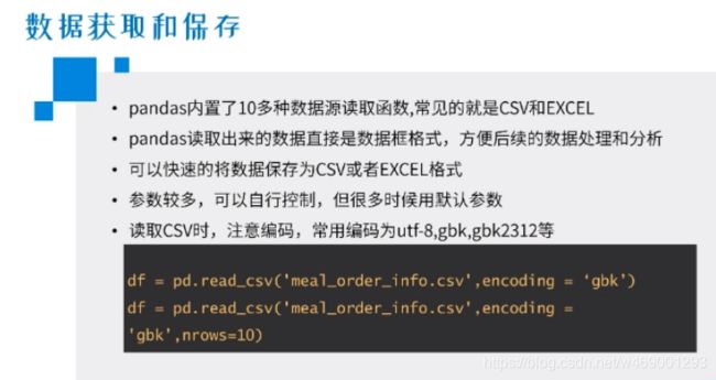
2. 数据获取和保存

• os.getcwd() #getcwd：获取当前的路径
• os.chdir(‘E:\Python learn\10 Python数据分析\第3章 Pandas数据分析运用’) #chdir：路径前缀
• df.head(5) #head：查看前5行
• df.tail(5) #head：查看最后5行
• df.dtypes #dtypes：查看每行的类型
• df = pd.read_csv(r’autoshop_store.csv’,encoding = ‘gbk’,
  dtype={‘id’:str,‘admin_id’:str}) #dtype：改变数据类型
• pd.__ version __ #pd的类型
• df = pd.read_csv(r’autoshop_store.csv’,encoding = ‘gbk’,
  dtype={‘id’:str,‘admin_id’:str}, nrows=10,
  sep=’,’) #sep：分隔符
• df = pd.read_csv(r’autoshop_store.csv’,encoding = ‘gbk’,
  dtype={‘id’:str,‘admin_id’:str}, nrows=10,
  sep=’,’,na_values=31) #na_values：缺失值,31变成NaN
• sheet_name = [‘autoshop_store’ + str(i) for i in range(1,4)] #工作表内容显示
• for i in sheet_name:
  data = pd.read_excel(‘autoshop_store1.xlsx’,encoding = ‘gbk’,
  sheet_name = i,dtype={‘id’:str,‘admin_id’:str})
  data_all = pd.concat([data_all,data],axis=0,ignore_index = True)
  #concat,ignore_index???
• #保存
  data_all.to_csv(‘data_all.csv’,index = False, encoding = ‘utf-8’)

3. 数据筛选

• order = pd.read_excel(‘autoshop_store1.xlsx’,encoding = ‘utf-8’,sheet_name=0,dtype={‘id’:str,‘admin_id’:str})
• order.columns #列名
• order.name #选择某个变量
• order[‘name’][:5] #选择列
• order[[‘id’,‘admin_id’,‘name’]][:5] #选择行
• #loc和iloc的用法
• order.loc[A,B] #A：行索引名称或者条件，列索引名称或者标签
• order.loc[order[‘order_id’]==2,[‘order_id’,‘admin_id’,‘name’]]
  #???
• order.iloc[:,1:4] #iloc：行索引位置，列索引位置

4. 条件查询和增删改查

• order[[‘id’,‘store_id’,‘addtime’,‘nickname’,]][order[‘store_id’] == 36]
  #获取’id’,‘store_id’,‘addtime’,'nickname’列，并’store_id’为36
• order[[‘id’,‘store_id’,‘addtime’,‘nickname’]][(order[‘store_id’] == 36) & (order[‘id’] > 124)]
• order[[‘id’,‘store_id’,‘addtime’,‘nickname’]][(order[‘store_id’] == 36) | (order[‘id’] > 124)]
• order[[‘id’,‘store_id’,‘addtime’,‘nickname’]][~(order[‘store_id’] == 36)]
• order[[‘id’,‘store_id’,‘addtime’,‘nickname’]][order[‘store_id’].between(10,30,inclusive=True)]
  #between：获取store_id为10-30，开合
• order[[‘id’,‘store_id’,‘addtime’,‘nickname’]][order[‘nickname’].isin([‘学者’,‘文’])]
  #isin：判断次数
• order[[‘id’,‘store_id’,‘addtime’,‘nickname’]][order[‘nickname’].str.contains(‘学’)]
  #str.contains：判断字符串包含
• order[‘ceshi1’] = order[‘id’] * order[‘id’] #增加列
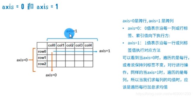
• order.drop(‘ceshi2’,axis=1,inplace = True)
  #axis=1,删除列，沿每一行或者列标签值执行
• order.insert(0,‘x1’,mid) #insert插入列
• order.drop(labels = [3,4], axis = 0) #labels：删除行
• order.loc[order[‘store_id’] == 11,‘store_id’] =11000 #loc：批量修改值
• order.rename(columns={‘x1’:‘y1’},inplace = True) #rename：更改列标签名
• order.rename(index={0:‘0000’},inplace = True) #rename：更改行索引名
• order.describe()
  #表统计：
  #count：个数；
  #mean：均值；
  #std：标准差；
  #min：最小值；
  #25%：25，50,75中位数
  #max：最大值
• order.describe().loc[‘count’] ==0 #True表示缺失
  

5. 数据库数据获取和保存

数据获取

• from sqlalchemy import create_engine
• create_engine(‘mysql+pymysql://user:passward@IP:3306/test01’)
• #建立连接
  conn = create_engine(‘mysql+pymysql://root:709623@localhost:3306/jupyter_notebook’)
• sql = ‘select * from autoshop_store’
• df1 = pd.read_sql(sql,conn)
• def query(table):
  host = ‘localhost’
  user = ‘root’
  passward = ‘709623’
  database = ‘jupyter_notebook’
  port = 3306
  conn = create_engine(‘mysql+pymysql://{}:{}@{}:{}/{}’.format(user,passward,host,port,database))
  sql = 'select * from ’ + str(‘autoshop_store’)
  results = pd.read_sql(sql,conn)
  return results
• df2 = query(‘autoshop_store’)

数据保存

• df = pd.read_csv(r’autoshop_store1.csv’,encoding = ‘gbk’)
• conn = create_engine(‘mysql+pymysql://root:709623@localhost:3306/jupyter_notebook’)
• try:
  df.to_sql(‘autoshop_store_1’,con = conn,index = False,if_exist=‘replace’)
  #命名表：autoshop_store_1
  #建立连接：con（to_sql中）
  #不用写索引：index = False
  #表存在：替换（replace）、追加（）、不加入（）
  except:
  print(‘error’)

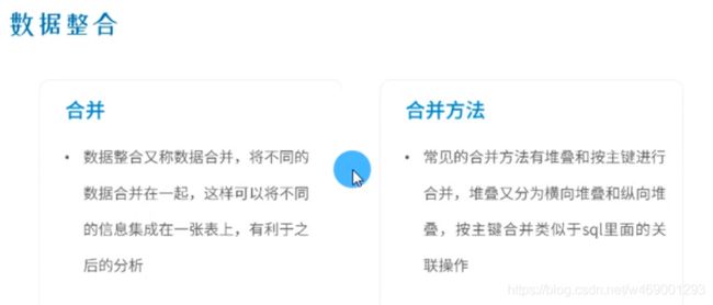
6. 数据整合

• df1 = pd.DataFrame({‘id’:[1,2,3,4,5],‘name’:[‘张三’,‘李四’,
  ‘王二’,‘丁一’,‘赵五’],‘age’:[27,24,25,23,25],‘gender’:[‘男’,‘男’,‘女’,‘男’,‘女’]})
• merged = pd.concat([df1,df2],axis=1,join=‘inner’) #inner：纵向交集
• merged = pd.concat([df1,df2],axis=1,join=‘outer’) #inner：纵向并集
• data = pd.concat([order1,order2,order3],axis=0,ignore_index = False)
  #ignore_index = False，索引不变
• data = pd.concat([order1,order2,order3],axis=0,ignore_index = True)
  #ignore_index = True，索引累加
• data.reset_index(drop = True,inplace = True) #重置索引
• mergel = pd.merge(left=df1,right=df2,how=‘right’,left_on=‘id’,right_on=‘Id’)
  #how链接方式
  #left_on：左边用什么做关联
  #right_on：右边用什么做关联
  #outer：全连接
  #inner：内连接
• mergel = pd.merge(left=df1,right=df2,how=‘inner’,left_on=‘id’,right_on=‘Id’)
  #sort = True，排序
• mergel = pd.merge(left=df1,right=df2,how=‘inner’,left_index=True,right_index=True)
  #left_index：按照索引合并
  

7. 层次化索引

• order = pd.read_excel(‘autoshop_store.xlsx’,encoding = ‘gbk’,sheet_name=0,header=0,
  index_col=[0,1]) #index_col：行索引
• order.loc[1].loc[1] #两次索引引用
• order.loc[(1,1),:] #两次索引引用
• order.loc[(1,[1]),:] #两次索引引用
• order.loc[(a,[b,c]),[‘d’,‘e’]]
• order.loc[(a,[b,c]),‘d’]
• order.loc[(a,[b,c]),[‘d’]]
  

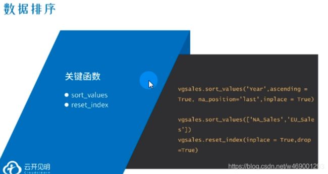
8. 数据排序

• vgsales.isnull() #isnull：判断是否缺失
• np.sum(vgsales.isnull(),asix=0) #判断空值的数
• vgsales.sort_values(‘admin_id’,ascending=True,na_position=‘last’,inplace=True)
  #asccending：True按升序排列,False按降序排列
  #na_position：last缺失值排最后,first缺失值排最前面
• vgsales.reset_index(drop=True,inplace=True) #索引重置
• vgsales.sort_values([‘A’,‘B’]) #A先升序，然后B再升序

9. 分组聚合

• vgsales = pd.read_excel(‘autoshop_user.xlsx’,encoding=‘gbk’)

• var_name = [‘id’,‘addtime’,‘store_id’]

• median #求中位数

• vgsales[var_name].min(axis=0) #max,median

• vgsales[var_name].cumsum(axis=0) #cumsum：累加

• vgsales[var_name].sum(axis=0) #总计

• vgsales[var_name].quantile([0,0.2,0.5,1]) #quantile：求中位数

• vgsales.describe() #describe：汇总

• vgsales.describe(include= [‘object’])
  #include= [‘object’]：计算统计量
  #count：总数
  #unique：元素值去重后数量
  #top：出现最多的元素值
  #freq：出现最多的元素值次数

• groupde.count() #统计个数

• groupde.size() #每个有几个样本

• groupde.median().loc[([1980,1986],‘Fighting’),:]

• groupde.agg([np.mean,np.sum]).head(5) #agg：聚合算法，mean，sum

• groupde.agg([np.mean,np.sum]).loc[[2,3],(‘addtime’,[‘mean’,‘sum’])]

• #自定义函数
  def DoubleSUM(data):
  s = data.sum()*2
  return s
  groupde.agg({‘addtime’:DoubleSUM})
  vgsales[var_name].apply(np.sum,axis=0) #apply
  vgsales[var_name].apply(lambda x: x[1] - x[2],axis=1) #第二列减去第三列

• #transform函数
  groupde.mean().transform(lambda x: x*2)

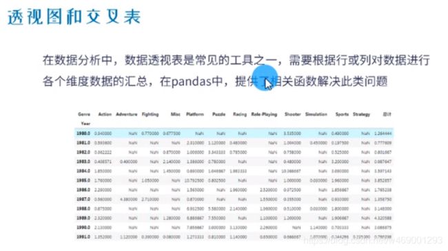
10. 透视图和交叉表

透视图

• pd.pivot_table(data=df,index=‘store_id’,columns=‘time’,values=‘id’,
  aggfunc=np.mean,margins=True,fill_value=0,margins_name=‘总计求均值’)
  #pivot_table：透视图，求均值、和
  #index：行标签
  #columns：列标签
  #values：值
  #aggfunc：聚合函数
  #mean：均值；
  #margins：是否需要总计
  #fill_value：空值为0
  #margins_name：总计名称
• pd.pivot_table(data=df,index=‘store_id’,columns=‘time’,values=‘id’,
  aggfunc=[np.sum,np.median],margins=True,fill_value=0,margins_name=‘总计求均值’).head(10)
• pd.pivot_table(data=df,index=[‘store_id’,‘time’],values=‘id’,
  aggfunc=[np.sum,np.median],margins=True,fill_value=0,margins_name=‘总计求均值’).head(50)

交叉表

• pd.crosstab(index=df[‘name’],columns=df[‘id’],margins=True)
  #crosstab：交叉表，求个数
• pd.crosstab(index=df2[‘name’],columns=df2[‘id’],normalize=‘all’,margins=True)
  #normalize=‘all’：每个值出现的百分比
• pd.crosstab(index=df2[‘name’],columns=df2[‘id’],normalize=‘index’,margins=True)
  #normalize=‘index’：行的百分比
• pd.crosstab(index=df2[‘name’],columns=df2[‘id’],normalize=‘columns’,margins=True)
  #normalize=‘index’：列的百分比
  

11. Pandas其他函数运用（日期 时间 变化率）

日期 时间

• sec_cars = pd.read_excel(‘autoshop_user2.xlsx’,encoding=‘gbk’,na_values=‘暂无’)
  #na_values：空
• sec_cars[‘time’] = pd.to_datetime(sec_cars[‘time’],format = ‘%Y-%m-%d’,errors=‘coerce’)
  #to_datetime：日期转化
  #coerce：空值
• sec_cars[‘price’].unique() #unique：有哪些取值
• sec_cars[‘price’].value_counts() #出现次数
• sec_cars[‘price’] = sec_cars[‘price’].str[:-1].astype(‘float’) #astype(‘float’)：去单位
• sec_cars[‘price’] = sec_cars[‘price’].str.replace(’–’,‘缺失值’) #替换
• sec_cars[‘diff_time’] = pd.datetime.today() - sec_cars[‘time’] #多少天
• sec_cars[‘diff_time’]/np.timedelta64(1,‘D’) #timedelta64(1,‘D’)：天
• sec_cars[‘diff_time’]/np.timedelta64(30,‘D’) #timedelta64(30,‘D’)：月
• (sec_cars[‘diff_time’]/np.timedelta64(1,‘D’)).astype(int) #去小数点
• sec_cars[‘diff_day’] = (sec_cars[‘diff_time’]/np.timedelta64(1,‘D’)).astype(int) #去小数点
• sec_cars[‘diff_year’] = pd.datetime.today().year - sec_cars[‘time’].dt.year

变化率

• df = pd.read_excel(‘autoshop_user2.xlsx’,dtype={‘telephone’:str,‘time’:‘datetime64’})
• df[‘telephone’] = df[‘telephone’].astype(str).apply(lambda x :x.replace(x[3:7],’****’))
  #apply
  #replace
  #手机号中间用星号（*号）
• df[‘email’] = df[‘email’].apply(lambda x: x.split(’@’)[1]) #split分隔
• df[‘new_tel’] = df[‘telephone’].str[0:3]
• df[‘telephone’].astype(str).apply(lambda x: x[0:3]) #取前三位
• data = df.sample(n = 1000,replace = False) #sample：抽样
• data[‘time’].dt.date #取日期
• data[‘time’].dt.time #取时间
• data[‘total_price’] = data[[‘quantity’,‘unitprice’]].apply(np.prod,axis=1) #prod：计算两个数相乘
• grouped_data = data.groupby(by = ‘time’).sum() #计算每天数据
• grouped_data.index = pd.to_datetime(grouped_data.index) #行索引转化为日期格式
• grouped_data[‘总价变化率’] = grouped_data[‘total_price’].pct_change() #总价变化率，下一行减上一上
• grouped_data[‘SMA_5’] = grouped_data[‘total_price’].rolling(5).mean() #计算5日的移动平均值
• grouped_data[‘SMA_10’] = grouped_data[‘total_price’].rolling(10).mean() #计算10日的移动平均值
• grouped_data[‘total_price_before’] = grouped_data[‘total_price’].shift(1)
  #shift(-1)向上平移一个单位
  #shift(1)向下平移一个单位
• (grouped_data[‘total_price’]-grouped_data[‘total_price’].shift(1))
• (grouped_data[‘total_price’].diff(1)

12. 重复值处理

• df.duplicated().head(10) #duplicated：判断行是否有无重复值
• df[df.duplicated(subset = [‘addtime’,‘nickname’],keep = ‘last’)].head(10) #subset：根据A.B值判断；keep：保留first（第一个），last（最后一个）
• np.sum(df.duplicated()) #duplicated：有多少重复值
• df.drop_duplicates().head(10) #drop_duplicates：删除重复值
• df[df.duplicated(subset = [‘addtime’,‘nickname’],inplace = True)].head(10)

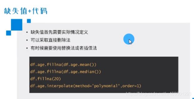
13. 缺失值处理

• df.isnull() #缺失值判断
• np.sum(df.isnull())
• np.sum(df.isnull(),axis = 1)
• df.apply(lambda x: sum(x.isnull()) /len(x),axis=0)
• df.dropna() #一行有一个缺失值，就会被删除
• df.dropna(how = ‘any’,axis=1) #一列有一个缺失值，就会被删除
• df.dropna(how = ‘all’,axis=1) #一列全部缺失，就会被删除
• df.telephone.fillna(df.telephone.mean()) #fillna：填充均值（median）或中位值（mean）
• df.telephone.mode()[0] #mode出现次数最多的元素
• df.fillna(method=‘ffill’) #method=‘ffill’：前项填充
• df.fillna(method=‘bfill’) #method=‘bfill’：后项填充
• df.telephone.interpolate(method=‘linear’) #interpolate(method=‘linear’)：差值法
• df.telephone.interpolate(method=‘polynomial’,order = 1) #差值，用的不多

14. 异常值处理

• xstd = df.unitprice.std() #std：标准差
• any(df.unitprice > xbar + 2*xstd) #判断有没有异常值
• Q1 = df.unitprice.quantile(q = 0.25) #下四分位数
• Q3 = df.unitprice.quantile(q = 0.75) #上四分位数
• IQR = Q3-Q1 #分位差
• any(df.unitprice > Q3 + 1.5*IQR) #True有异常值
• UL = Q3 + 1.5 * IQR
• replace_value = df.unitprice[df.unitprice < UL].max()
• df.loc[df.unitprice > UL,‘unitprice’] = replace_value
• P1 = df.unitprice.quantile(0.01)
• P99 = df.unitprice.quantile(0.99)
• df[‘unitprice_new’] = df[‘unitprice’]
• df.loc[df[‘unitprice’] > P99,‘unitprice_new’] = P99
• df.loc[df[‘unitprice’] < P1,‘unitprice_new’] = P1

15. 数据离散化

• df[‘unitprice_bin’] = pd.cut(df[‘unitprice’],4,labels=range(1,5)) #等宽分段
• pd.qcut(df[‘unitprice’],w,labels = range(0,4)) #qcut：等平分段
• df[‘unitprice_bin’] = pd.cut(df[‘unitprice’],w1,labels = range(0,4)) #等平分段