图像各向异性扩散（一）

百度百科上说：各向同性和各向异性是指物理性质在不同的方向进行测量得到的结论，如果物理性质和取向密切相关，不同取向的测量结果迥异，就称为各向异性。

1 图像向异性扩散滤波介绍

向异性扩散滤波通过是用来对图像实现平滑操作的。而在图像处理中，主要有高斯滤波相对应，与跨尺度的高斯平滑相比，它可以更好地保留生成的尺度空间表示中的边缘和纹理细节，且可以增强图像边缘。而高斯模糊不考虑对象的自然边界，并且对细节和噪声进行相同程度的平滑，降低了图像的定位精度和清晰度。

通常我们有将图像看作矩阵的。而将各向异性扩散是将图像看作热量场。每个像素看作热流，根据当前像素和周围像素的关系，来确定是否要向周围扩散。比如某个邻域像素和当前像素差别较大，表示这个邻域像素很可能是个边界，那么当前像素就不向这个方向扩散了，这个边界也就得到保留了。

---

各向异性扩散滤波的主要公式：

其中，I表示图像，t表示迭代次数。

四个散度公式是在四个方向上对当前像素求偏导，公式如下：

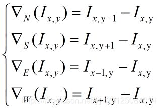
cN、cS、cE、cW代表四个方向上的导热系数，边界的导热系数都较小，公式如下：

 

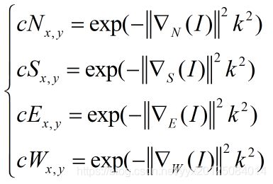
其中，系数k，取值越大越平滑，越不易保留边缘；lambda同样也是取值越大越平滑

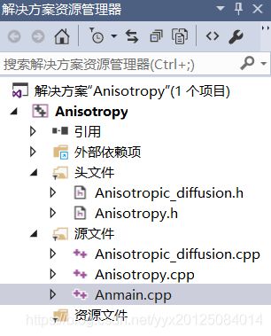
2 代码实现

    工程文件组织形式如下图所示：

2.1 main函数代码

（Anmain.cpp文件）

//         实现各向异性的图像扩散  实例代码
//         作者：yyx
//         时间：2019.11.9

#include 
#include 

#include "Anisotropy.h"
#include "Anisotropic_diffusion.h"

using namespace std;
using namespace cv;

char* create = "Theashold";
char* ThName = "result01";
int Theashold_value = 15;
int Theashold_max = 80;
void threshold_Callback(int, void*);
double lambda = 2.5;
float N = 20;

Mat src;

int main()
{
	src = imread("D:\\Code\\ImagesDataes\\data\\home.jpg", 1);
	if (!src.data)
	{
		printf("Could not find load image. \n");
		return -1;
	}
	namedWindow("input image", CV_WINDOW_AUTOSIZE);
	imshow("input image", src);
	cout << "作者：yyx" << "       " << "时间：2019.11.9" << endl;

	double t01 = getTickCount();
	vector mv;
	vector results;
	split(src, mv);
	for (int n = 0; n < mv.size(); n++) {
		Mat m = Mat::zeros(src.size(), CV_32FC1);
		mv[n].convertTo(m, CV_32FC1);
		results.push_back(m);
	}
	int w = src.cols;
	int h = src.rows;
	Mat copy = Mat::zeros(src.size(), CV_32FC1);

	for (int i = 0; i < N; i++) {
		anisotropy(results[0], copy);
		copy.copyTo(results[0]);
		anisotropy(results[1], copy);
		copy.copyTo(results[1]);
		anisotropy(results[2], copy);
		copy.copyTo(results[2]);
	}
	normalize(results[0], results[0], 0, 255, NORM_MINMAX);  //normalize归一化函数
	normalize(results[1], results[1], 0, 255, NORM_MINMAX);
	normalize(results[2], results[2], 0, 255, NORM_MINMAX);
	results[0].convertTo(mv[0], CV_8UC1);
	results[1].convertTo(mv[1], CV_8UC1);
	results[2].convertTo(mv[2], CV_8UC1);
	double t02 = getTickCount();

	//************************
	//  1 对图像进行平滑
	//************************
	Mat output;
	merge(mv, output);            //将多个单通道图像合成一幅多通道图像
	cout << " 图像扩散结果1所花费的时间：  " << (t02 - t01) / getTickFrequency() * 1000 << " s " << endl;
	imshow(ThName, output);
	imwrite("result01.jpg", output);

	//************************
	//  2 对图像进行平滑
	//************************

	namedWindow("result02", CV_WINDOW_AUTOSIZE);
	createTrackbar(create, "result02", &Theashold_value, Theashold_max, threshold_Callback);
	threshold_Callback(0,0);
	//Mat dst2 = src.clone();   // 虚拟克隆
	//double t1 = getTickCount();
	//anisotropic_diffusion(dst2, src, Theashold_value, lambda);
	//double t2 = getTickCount();
	//cout <<  " 图像扩散结果2所花费的时间：  "  << (t2 - t1) / getTickFrequency() * 1000 <<" s "<< endl;
	//imshow("result02", dst2);
	//imwrite("result02.jpg", dst2);


	waitKey(0);
	return 0;
}

void threshold_Callback(int, void*) {
	Mat dst2 = src.clone();   // 虚拟克隆
	double t1 = getTickCount();
	anisotropic_diffusion(dst2, src, Theashold_value, lambda);
	imshow("result02", dst2);
	double t2 = getTickCount();
	cout << " 图像扩散结果2所花费的时间：  " << (t2 - t1) / getTickFrequency() * 1000 << " s " << endl;
	cout<<"数值 K 的不同值："<< Theashold_value<

2.2 Anisotropy

Anisotropy.h文件

#pragma once
#ifndef _Anisotropy_h_
#define _Anisotropy_h_

#include 
#include 

using namespace std;
using namespace cv;

//  四邻域系数计算
void anisotropy(Mat &image, Mat &result);

#endif // _Anisotropy_h_

 Anisotropy.cpp文件

#include 
#include 

#include "Anisotropy.h"

using namespace std;
using namespace cv;

double  k = 15;

//  四邻域系数计算
void anisotropy(Mat &image, Mat &result) {
	int width = image.cols;
	int height = image.rows;
	// 四邻域梯度  
	float n = 0, s = 0, e = 0, w = 0;
	// 四邻域系数  
	float nc = 0, sc = 0, ec = 0, wc = 0;

	float k2 = k*k;
	float lambda2 = 0.25;
	for (int row = 1; row < height - 1; row++) {
		for (int col = 1; col < width - 1; col++) {
			// gradient  
			n = image.at(row - 1, col) - image.at(row, col);
			s = image.at(row + 1, col) - image.at(row, col);
			e = image.at(row, col - 1) - image.at(row, col);
			w = image.at(row, col + 1) - image.at(row, col);
			nc = exp(-n*n / k2);
			sc = exp(-s*s / k2);
			ec = exp(-e*e / k2);
			wc = exp(-w*w / k2);
			result.at(row, col) = image.at(row, col) + lambda2*(n*nc + s*sc + e*ec + w*wc);
		}
	}
}

2.3 Anisotropic_diffusion

Anisotropic_diffusion.h文件

#pragma once
#ifndef _Anisotropy_diffusion_h_
#define _Anisotropic_diffusion_h_

#include 
#include 

using namespace std;
using namespace cv;

void anisotropic_diffusion(Mat &out, Mat &in, int k, float lambda);

#endif //_Anisotropic_diffusion_h_

Anisotropic_diffusion.cpp文件

#include 
#include 

#include "Anisotropic_diffusion.h"

using namespace std;
using namespace cv;

void anisotropic_diffusion(Mat &out, Mat &in, int k, float lambda) {
	int i, j;
	int iter = 20;
	int nRow = in.rows, nCol = in.cols;
	float ei, si, wi, ni;
	float ce, cs, cw, cn;

	Mat tmp = in.clone();
	uchar *pin = in.data;
	uchar *ptmp = tmp.data;
	uchar *pout = out.data;

	for (int n = 0; n < iter; n++)
	{
		for (i = 1; i < nRow - 1; i++)
			for (j = 1; j < nCol - 1; j++)
			{
				float cur = ptmp[i*nCol + j];
				ei = ptmp[(i - 1)*nCol + j] - cur;
				si = ptmp[i*nCol + j + 1] - cur;
				wi = ptmp[(i + 1)*nCol + j] - cur;
				ni = ptmp[i*nCol + j - 1] - cur;

				ce = exp(-ei*ei / (k*k));
				cs = exp(-si*si / (k*k));
				cw = exp(-wi*wi / (k*k));
				cn = exp(-ni*ni / (k*k));

				//pout[i*nCol + j] = cur + lambda*(ce*ei + cs*si + cw*wi + cn*ni);
				pout[i*nCol + j] = cur + lambda*(ce + cs + cw + cn);
			}
		out.copyTo(tmp);
	}
}

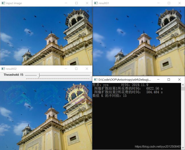
3 运行结果如下：

4 结论

对于图像的各向异性扩散的研究，现在只是粗浅地进行尝试，后边会继续深入。

 

注：全部工程Code放到我的百度云盘里面了，需要的自行下载。

链接：https://pan.baidu.com/s/1E0VYJqTDQIT0Y3eeccgoyQ
提取码：a39h