Attention机制梳理（三）——What is Attention in CV？

  现在NLP中很火的attention机制，其实早在14年Google-DeepMind的Compution Vision文章——Recurrent Models of Visual Attention中出现过了，15年的时候我曾做过一个ppt，介绍这篇文章，现在找不到了。这里我们通过重新梳理，希望能够搞清楚Attention的来龙去脉，有助于加深我们对Attention机制的理解。

How attention proposed in CV?

---

CNN在分类任务中的缺点

  14年GoogLeNet把图像分类任务推到了一个新高度，GoogLeNet是基于CNN技术实现的一种深层网络结构。但是，CNN通常使用固定大小的向量作为输入，这有几个缺点：

• 如果输入图片大小过大，要么通过resize到固定大小，要么cut出若干patch作为输入。resize操作会造成图片细节的丢失，而cut出若干个patch会造成计算量线性增加
• CNN本身具备一定的空间转换不变性，但当图像存在噪声或者目标部分遮挡时，CNN模型难以得到满意的结果

---

location-wise hard attention mechanism的具体做法

  于是Recurrent Models of Visual Attention提出使用location-wise hard attention mechanism进行RNN-based的图像分类。其具体做法是从输入图片中随机选择一个子区域去预测一个中间结果，模型既会预测图像标签，还可以定位目标的位置。也就是说attention based RNN model将图像分类和目标检测整合到了一个端到端的模型中。

---

location-wise hard attention mechanism的优势

  location-wise hard attention mechanism相比CNN-based的目标检测网络什么优势呢？
  CNN处理目标检测任务时，必须使用一个单独的网络去预测潜在的目标位置，然后对这些位置进行分类，潜在的目标位置往往很多，导致inference的代价非常高。

---

Why RNN-based Attention, not others?

作为早期CV-attention的开山经典之作，为什么会选择通过RNN完成Attention呢？

• 以前的目标检测任务，通过分类级联减少滑窗数量，或者提高候选框中有目标存在的准确率的方法，去进行加速，但“预测候选框+分类”的框架对目标检测任务的提升帮助有限。
• 显著性检测是基于人类感知提出来的一类任务，它通过局部低维特征找出潜在感兴趣的显著性区域，确实可以捕获人眼移动的一些属性，但是显著性检测的计算量很大，且只关注图像的低维语义，忽略了场景或任务需求的内容语义。
• 也有一些方法像本文一样，将CV视为 a sequential decision task ，本文的做法就是将图像信息序列化地进行聚集，然后基于上一次得到的位置fixation，去决定下一次要关注的区域。有文章采用learned Bayesian observer mode进行目标检测，也有方法跟我们一样采样了a policy gradient formulation(策略梯度假设)，但是其限制条件比我们更加严格，且系统只学到了一部分内容。

  跟本文最接近的，采用Attention化处理（attentional processing）的深度学习文章有以下三篇，可见本文提出的Glimpse Network并非空穴来风，本文的构想是采用RNN在时序上将视觉信息进行聚合，然后决定下一步采取什么动作。学习过程可以实现对序列决策处理的端到端优化，并不需要像以前的目标检测方法那样依赖于greedy action selection。

• 2012年-Learning where to attend with deep architectures for image tracking
• 2010年-Learning to combine foveal glimpses with a third-order boltzmann machine
• 2014年-On Learning Where To Look

---

What is Recurrent Attention Model?

参考资料

• 基于Attention的图片分类、图片生成、图片主题生成、字符识别：Attention Model介绍很不错的博客
• cosmosshadow.com：很好的网站，总结了很多CS、Math和ML的东西
• 注意力机制之Recurrent Models of Visual Attention：记录了RAM公式的详细推导，是所有博客里推导最好理解的。
• RAM： Recurrent Models of Visual Attention 学习笔记：包括论文解析、Torch代码和、TF实践
• 【深度学习】聚焦机制DRAM(Deep Recurrent Attention Model)算法详解：从数学推导的角度，介绍DRAM的原理
• 【增强学习】Recurrent Visual Attention源码解读：结合torch代码，解读RAM的网络结构

模型

基于Attention的图片分类、图片生成、图片主题生成、字符识别博客已经介绍的很清楚了，这里引用过来

1. Glimpse Sensor: 在t步，图片$x_t$的$l_{t-1}$位置处取不同大小的区域，组合成数据$\rho \left(x_t,l_{t-1}\right)$
2. Glimpse Network: 将图片局部信息与位置信息整合成$g_t$
3. Model Architecture: $h_{t-1}$为隐藏记忆单元，每轮加入新的KaTeX parse error: Expected '}', got 'EOF' at end of input: g_{t)，生成新的$h_t$，并以此生成感兴趣的at与新的位置$l_t$
   
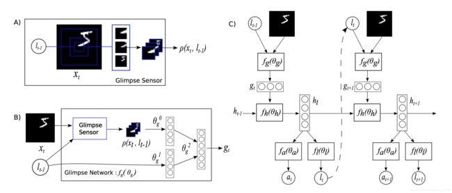
   下面对Glimpse Sensor、Glimpse Network和Model Architecture作更详细的解释。（引用自）

• 图A：此部分称之为Glimpse Sensor，也就是感应器，其实就是给定一个图片的location（坐标，这个坐标为中心），采集一副大的图片的子图，因为使用的MNIST的图片，所以只有一个通道，黑白。另外，采集图片的尺寸不一样，有的图片采集的scale更大，从A中来看是采集了三个size的图片，然后进行sub-smapling获得统一尺寸的图片8x8（在Torch代码中，这个下采样图片个数变成了2）所以输入的locator（定位器）$l_{t+1}$和整副图片$x_t$，得到了进行采样之后的n个子图片表达 $\rho \left(x_t,l_{t-1}\right)$。
• 图B：总的输出是$g_t$，由两部分的feature进行连接得到。其中${\theta }_g^0$是由图A中的$\rho$通过一个linear regression得到, ${\theta }_g^1$是由locator通过linear regression得到。
• 图C：这里面有一个RNN，图B得到的$g_t$通过了linear regression，ReLU得到，然后$g_t$通过linear regression得到$f_h$（RNN中的hidden layer，可以用于下一次的输入以及当前的输出），然后将$h_t$通过locator的网络，用于计算下一个输入的locator（具体操作看下一个section）。在这个网络里面，和普通RNN会有些不同，普通的RNN是不会把输出$l_{t-1}$和hidden layer同时保留进行计算的，一般是保留一个。这里要注意的就是$l_{t-1}$这部分的权值更新是没有监督学习的，只是根据reward进行gradient ascent。就是让这部分的权重更新的方向是更加接近positive reward。如果是negative reward就远离。

How to train like a Markov Decision Process?

由于本文的主要目的并非着重介绍RAM这篇文章，因此训练反向传导公式的推导引用自注意力机制之Recurrent Models of Visual Attention，并对其中缺失的推导细节做了补充

梯度推导的整体流程

  整个模型过程可以看做是一个局部马尔科夫决策过程。每个阶段的动作和位置只与上一阶段的动作和位置有关。即展开RNN结构，以时间为序，整个过程可表示为
$$s_{1:t}=x_1,l_1,a_1,\dots ,x_{t-1},l_{t-1},a_{t-1},x_t$$  根据上一阶段的动作$a_t$和位置$l_{t-1}$，从输入图像提取出信息，通过模型网络，输出特征信息，利用POMDP决定出下一阶段的动作$a_t$和位置$l_{t-1}$，设：

• $\pi \left(a_t|s_{1:t};\theta \right)$为参数化为$\theta$的随机策略；
• $p\left(l_0\right)$为初始位置的概率；
• $p\left(s_{t+1}|s_{1:t};a_t\right)$为执行动作$a_t$，位置由$l_t$到$l_{t+1}$的概率；
• $r\left(s_{1:t},a_t,s_{t+1}\right)$表示执行动作$a_t$，位置由$l_t$到$l_{t+1}$的奖励；
• ${\gamma }^t$表示奖励的折扣。

  则整个过程的回报： $R(s)={\sum }_{t=1}^T{\gamma }^{t}r\left(s_{1:t},a_t,s_{t+1}\right)$
  策略参数$\theta$的期望回报为:
$$J(\theta )=E_{p(s|\theta )}[R(s)]=\int p(s|\theta )R(s)\mathrm{d}s$$$$p(s|\theta )=p\left(l_0\right)\prod _{t=1}^{T}p\left(s_{t+1}|s_{1:t},a_t\right)\pi \left(a_t|s_{1:t},\theta \right)$$  对于梯度计算，有个log小技巧， $\nabla p(s|\theta )=p(s|\theta )\nabla \log p(s|\theta )$故计算回报的梯度有:
$${\nabla }_{\theta }J(\theta )=\int {\nabla }_{\theta }p(s|\theta )R(s)\mathrm{d}s$$$$=\int p(s|\theta ){\nabla }_{\theta }\log p(s|\theta )R(s)\mathrm{d}s$$$$=\int p(s|\theta )\sum _{t=1}^T{\nabla }_{\theta }\log \pi \left(a_t|s_{1:t};\theta \right)R(s)\mathrm{d}s$$$$=E_{p(s|\theta )}\left[\sum _{t=1}^T{\nabla }_{\theta }\log \pi \left(a_t|s_{1:t};\theta \right)R(h)\right]$$
  由于$p(s|\theta )$未知，故取经验平均求解，即：
$${\nabla }_{\theta }J\widehat{(\theta )}=\frac{1}{M}\sum _{i=1}^M\sum _{t=1}^T{\nabla }_{\theta }\log \pi \left(a_t^i|s_{1:t}^i;\theta \right)R_t^i$$
  可以通过减去一个$b_t$降低方差，即：
$$\frac{1}{M}\sum _{i=1}^M\sum _{t=1}^T{\nabla }_{\theta }\log \pi \left(a_t^i|s_{1:t}^i;\theta \right)\left(R_t^i-b_t\right)$$
  $b_t$可取$E_{\pi }\left[R_t\right]$，该算法被称为REINFORCE。
  训练神经网络自然想到反向传播，通过REINFORCE得到$f_a$和$f_l$的梯度信息。然后反向依次训练RNN，Glimpse Network。对于分类问题，由于$a_T$是确定，最大化$\log \pi \left(a_T|s_{1:T};\theta \right)$，通过优化$f_a$的交叉熵得到梯度，反向训练模型。

梯度推导的补充

${\nabla }_{\theta }\log p(s|\theta )={\sum }_{t=1}^T{\nabla }_{\theta }\log \pi \left(a_t|s_{1:t};\theta \right)$的推导：

对$p(s|\theta )=p\left(l_0\right){\prod }_{t=1}^{T}p\left(s_{t+1}|s_{1:t},a_t\right)\pi \left(a_t|s_{1:t},\theta \right)$两边求$\log$，得:
$$\log p(s|\theta )=\log p(l_0)+\sum _{t=1}^T\log (p\left(s_{t+1}|s_{1:t},a_t\right)\pi \left(a_t|s_{1:t},\theta \right))$$   为了让公式看的更清楚，将$p\left(s_{t+1}|s_{1:t},a_t\right)$简写成$p\left(s_{t+1}|t\right)$，将$\pi \left(a_t|s_{1:t},\theta \right)$简写成$\pi \left(a_t|t,\theta \right)$，代入上式得到，同时对两边求梯度$\nabla$，得：
$$\nabla \log p(s|\theta )=\nabla \log p(l_0)+\nabla \sum _{t=1}^T\log (p\left(s_{t+1}|t\right)\pi \left(a_t|t,\theta )\right)$$   注意，这里$\log p\left(l_0\right)$是跟t和$\theta$无关的常量，求导后为0，消去$\log p\left(l_0\right)$后，得：
$$\nabla \log p(s|\theta )=\nabla \sum _{t=1}^T\log (p\left(s_{t+1}|t\right)\pi \left(a_t|t,\theta \right))$$   利用$\log (ab)=\log a+logb$将上式右边展开得，
$$\nabla \log p(s|\theta )=\nabla (\sum _{t=1}^T(\log (p\left(s_{t+1}|t\right)+\log (\pi \left(a_t|t,\theta \right))))$$   考虑到$\log (p\left(s_{t+1}|t\right)$为常数，求导后为0，故可消除，得：
$$\nabla \log p(s|\theta )=\nabla (\sum _{t=1}^T(\log (\pi \left(a_t|t,\theta \right))))$$  将$\nabla$移到$\sum$里面，再加上$\theta$角标，得:
$$\nabla \log p(s|\theta )=\sum _{t=1}^T(\nabla \log (\pi \left(a_t|t,\theta \right)))$$  最后，将$\pi \left(a_t|t,\theta \right)$替换回$\pi \left(a_t|s_{1:t},\theta \right)$，得:
$$\nabla \log p(s|\theta )=\sum _{t=1}^T(\nabla \log (\pi \left(a_t|s_{1:t},\theta \right)))$$  至此，完成推导。

R替换成R-b的作用

这里的主要作用是为了减少方差，VR(Variance Reduction)方法以及其中的baseline都是增强学习中的基本设置。更多理解，待后续补上强化学习的知识之后，再来分析。

源码分析

请参考【增强学习】Recurrent Visual Attention源码解读：结合torch代码，解读RAM的网络结构