3.8激活函数【relu sigmoid tanh 】

学习来源

1 ReLU函数

ReLU（rectified linear unit）函数提供了一个很简单的非线性变换。给定元素x，该函数定义为:
$$ReLU(x)=max(x,0)$$

ReLU函数只保留正数元素，并将负数元素清零。

为了直观地观察激活函数变换，我们先定义一个绘图函数xyplot。

%matplotlib inline
import torch
import numpy as np
import matplotlib.pylab as plt
import sys
sys.path.append("..") 
import d2lzh_pytorch as d2l

def xyplot(x_vals, y_vals, name):
    d2l.set_figsize(figsize=(5, 2.5))
    plt.plot(x_vals.detach().numpy(), y_vals.detach().numpy())
    plt.xlabel('x')
    plt.ylabel(name + '(x)')

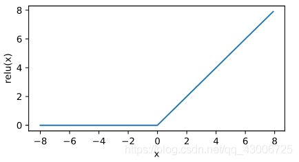
接下来通过Tensor提供的relu函数来绘制ReLU函数。可以看到，该激活函数是一个两段线性函数。

x = torch.arange(-8.0, 8.0, 0.1, requires_grad=True)
y = x.relu()
xyplot(x, y, 'relu')

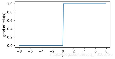
#绘制ReLU函数的导数。

y.sum().backward()
xyplot(x, x.grad, 'grad of relu')

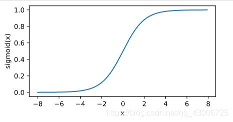
2 sigmoid函数

sigmoid函数可以将元素的值变换到0和1之间：
$$sigmoid(x)=\frac{1}{exp(-x)}$$

y = x.sigmoid()
xyplot(x, y, 'sigmoid')

依照链式法则，sigmoid函数的导数为
$$sigmoi{d}^{{}^{\prime }}(x)=sigmoid(x)(1-sigmoid(x))$$

#下面绘制了sigmoid函数的导数。
#当输入为0时，sigmoid函数的导数达到最大值0.25；当输入越偏离0时，sigmoid函数的导数越接近0。
x.grad.zero_()    #梯度清零
y.sum().backward()
xyplot(x, x.grad, 'grad of sigmoid')

3 tanh函数

tanh（双曲正切）函数可以将元素的值变换到-1和1之间：
$$tanh(x)=\frac{1-exp(-2x)}{1+exp(-2x)}$$

#我们接着绘制tanh函数。
#当输入接近0时，tanh函数接近线性变换。虽然该函数的形状和sigmoid函数的形状很像，但tanh函数在坐标系的原点上对称。
y = x.tanh()
xyplot(x, y, 'tanh')

[外链图片转存失败,源站可能有防盗链机制,建议将图片保存下来直接上传(img-OczPGbCz-1590111876321)(output_10_0.svg)]

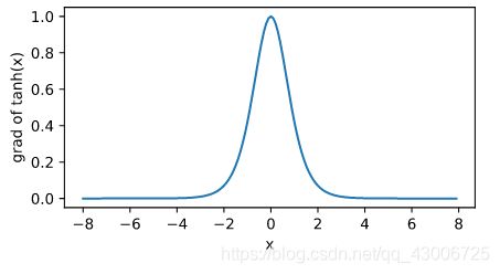
依据链式法则，tanh函数的导数
$$tan{h}^{\prime }(x)=1-tan{h}^2(x)$$

下面绘制了tanh函数的导数。当输入为0时，tanh函数的导数达到最大值1；当输入越偏离0时，tanh函数的导数越接近0。

x.grad.zero_()
y.sum().backward()
xyplot(x, x.grad, 'grad of tanh')