opencv中grabcut算法解读
- opencv库函数:
grabCut( InputArray _img, InputOutputArray _mask, Rect rect, InputOutputArray _bgdModel, InputOutputArray _fgdModel, int iterCount, int mode )
参数说明:
- img——待分割的源图像,必须是8位3通道(CV_8UC3)图像,在处理的过程中不会被修改;
- mask——掩码图像,如果使用掩码进行初始化,那么mask保存初始化掩码信息;在执行分割的时候,也可以将用户交互所设定的前景与背景保存到mask中,然后再传入grabCut函数;在处理结束之后,mask中会保存结果。mask只能取以下四种值:
GC_BGD(=0),背景;
GC_FGD(=1),前景;
GC_PR_BGD(=2),可能的背景;
GC_PR_FGD(=3),可能的前景。
- rect——用于限定需要进行分割的图像范围,只有该矩形窗口内的图像部分才被处理;
- bgdModel——背景模型,如果为null,函数内部会自动创建一个bgdModel;bgdModel必须是单通道浮点型(CV_32FC1)图像,且行数只能为1,列数只能为13x5;
- fgdModel——前景模型,如果为null,函数内部会自动创建一个fgdModel;fgdModel必须是单通道浮点型(CV_32FC1)图像,且行数只能为1,列数只能为13x5;
- iterCount——迭代次数,必须大于0;
- mode——用于指示grabCut函数进行什么操作,可选的值有:
GC_INIT_WITH_RECT(=0),用矩形窗初始化GrabCut;
GC_INIT_WITH_MASK(=1),用掩码图像初始化GrabCut;
GC_EVAL(=2),执行分割。
- 函数:
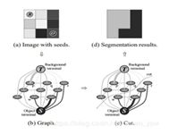
grabcut算法是一种基于图论的图像分割方法,首先要定义一个Gibbs能量函数,然后求解这个函数的min-cut,这个min-cut就是前景背景的分割像素集合。
能量函数的定义 :
![]()
其中U函数部分表示能量函数的区域数据项,V函数表示能量函数的光滑项(边界项)。

- k-means算法:
- K-means算法的相关描述:
聚类是一种无监督的学习,它将相似的对象归到同一簇中。聚类的方法几乎可以应用所有对象,簇内的对象越相似,聚类的效果就越好。K-means算法中的k表示的是聚类为k个簇,means代表取每一个聚类中数据值的均值作为该簇的中心,或者称为质心,即用每一个的类的质心对该簇进行描述。
聚类和分类最大的不同在于,分类的目标是事先已知的,而聚类则不一样,聚类事先不知道目标变量是什么,类别没有像分类那样被预先定义出来,所以,聚类有时也叫无监督学习。
聚类分析试图将相似的对象归入同一簇,将不相似的对象归为不同簇,那么,显然需要一种合适的相似度计算方法,我们已知的有很多相似度的计算方法,比如欧氏距离,余弦距离,汉明距离等。事实上,我们应该根据具体的应用来选取合适的相似度计算方法。
K-means算法虽然比较容易实现,但是其可能收敛到局部最优解,且在大规模数据集上收敛速度相对较慢。
- K-means算法的工作流程:
- 随机确定k个初始点的质心。
- 将数据集中的每一个点分配到一个簇中,即为每一个点找到距其最近的质心,并将其分配给该质心所对应的簇。
- 每一个簇的质心更新为该簇所有点的平均值。
- 重复1~3步骤直到质心收敛或则是最大迭代次数。

- 最小割与最大流算法(mincut & maxflow)
- 首先介绍Mincut问题:
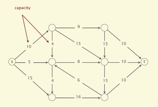
一个有向图,并有一个源顶点(source vertex)和目标顶点(target vertex).边的权值为正,又称之为容量(capacity).如下图:

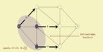
一个st-cut(简称割cut)会把有向图的顶点分成两个不相交的集合,其中s在一个集合中,t在另外一个集合中(在图像分割中,你可以将s理解成前景,t理解成背景)。
这个割的容量(capacity of the cut)就是A到B所有边的容量和。注意这里不包含B到A的。参见下面几幅图。最小割问题就是要找到割容量最小的情况。
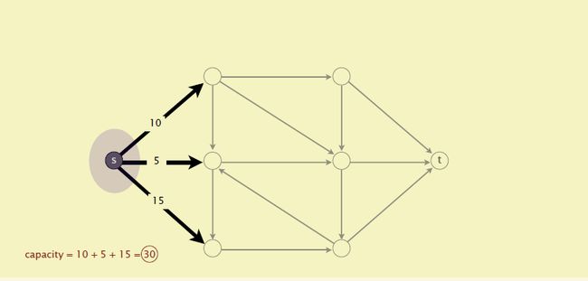

可以想象成某某国家要控制网络,使得国民不能跟外面联络,S代表某个国家,t代表其余的世界。而每条边上代表着是带宽,带宽越大,肯定建设成本也越大,在进行cut的时候当然希望能达到完全断开的效果但又能破坏越少的基建设施,这就是最小割问题。
- Maxflow
接着介绍maxflow问题。跟mincut问题类似,maxflow要处理的情况也是一个有向图,并有一个原顶点(source vertex)和目标(target vertex).边的权值为正,又称之为容量(capacity).如下图:
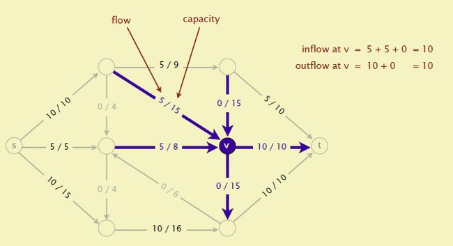
一个st-flow(简称flow)是为每条边附一个值,这个值需要满足两个条件:
- 0<=边的flow <<边的capacity
- 除了s和t外,每个顶点的inflow要等于outflow
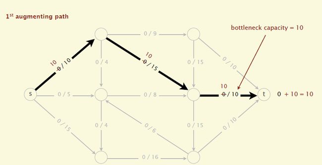
见下图,其实这个很好理解,可以想象成水管或者电流,一个flow的值(value of the flow)就是t的inflow.Maxflow就是找到这个最大值。


后面会发现Mincut和maxflow的问题是对偶的,解出了maxflow也就知道了mincut的解。现在先介绍一种解maxflow的算法Ford-Fulkerson,为了方便,简称FF算法。
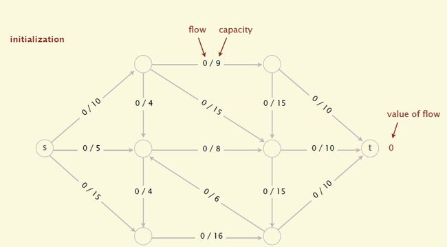
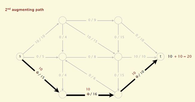
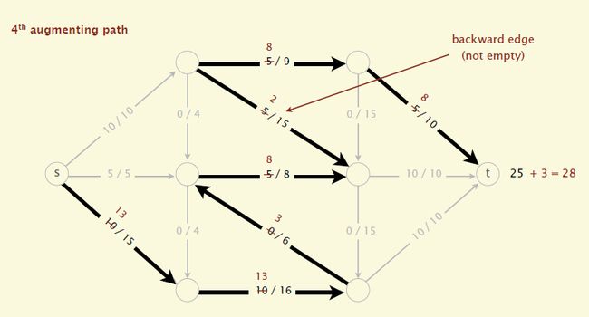
(1)初始化,所有边的flow都初始化为0
(2)沿着增广路径增加flow。增广路径是一条从s到t的无向路径,但也有些条件,可以经过没有满容量的前向路径(s到t)或者是不为空的反向路径(t->s)


grabcut.cpp:
/*M///
//
// IMPORTANT: READ BEFORE DOWNLOADING, COPYING, INSTALLING OR USING.
//
// By downloading, copying, installing or using the software you agree to this license.
// If you do not agree to this license, do not download, install,
// copy or use the software.
//
//
// Intel License Agreement
// For Open Source Computer Vision Library
//
// Copyright (C) 2000, Intel Corporation, all rights reserved.
// Third party copyrights are property of their respective owners.
//
// Redistribution and use in source and binary forms, with or without modification,
// are permitted provided that the following conditions are met:
//
// * Redistribution's of source code must retain the above copyright notice,
// this list of conditions and the following disclaimer.
//
// * Redistribution's in binary form must reproduce the above copyright notice,
// this list of conditions and the following disclaimer in the documentation
// and/or other materials provided with the distribution.
//
// * The name of Intel Corporation may not be used to endorse or promote products
// derived from this software without specific prior written permission.
//
// This software is provided by the copyright holders and contributors "as is" and
// any express or implied warranties, including, but not limited to, the implied
// warranties of merchantability and fitness for a particular purpose are disclaimed.
// In no event shall the Intel Corporation or contributors be liable for any direct,
// indirect, incidental, special, exemplary, or consequential damages
// (including, but not limited to, procurement of substitute goods or services;
// loss of use, data, or profits; or business interruption) however caused
// and on any theory of liability, whether in contract, strict liability,
// or tort (including negligence or otherwise) arising in any way out of
// the use of this software, even if advised of the possibility of such damage.
//
//M*/
#include "precomp.hpp"
#include "gcgraph.hpp"
#include
using namespace cv;
/*
This is implementation of image segmentation algorithm GrabCut described in
"GrabCut — Interactive Foreground Extraction using Iterated Graph Cuts".
Carsten Rother, Vladimir Kolmogorov, Andrew Blake.
*/
/*
GMM - Gaussian Mixture Model
*/
class GMM
{
public:
static const int componentsCount = 5;
GMM( Mat& _model );
double operator()( const Vec3d color ) const;
double operator()( int ci, const Vec3d color ) const;
int whichComponent( const Vec3d color ) const;
void initLearning();
void addSample( int ci, const Vec3d color );
void endLearning();
private:
void calcInverseCovAndDeterm( int ci );
Mat model;
double* coefs;
double* mean;
double* cov;
double inverseCovs[componentsCount][3][3]; //协方差的逆矩阵
double covDeterms[componentsCount]; //协方差的行列式
double sums[componentsCount][3];
double prods[componentsCount][3][3];
int sampleCounts[componentsCount];
int totalSampleCount;
};
//背景和前景各有一个对应的GMM(混合高斯模型)
GMM::GMM( Mat& _model )
{
//一个像素的(唯一对应)高斯模型的参数个数或者说一个高斯模型的参数个数
//一个像素RGB三个通道值,故3个均值,3*3个协方差,共用一个权值
const int modelSize = 3/*mean*/ + 9/*covariance*/ + 1/*component weight*/;
if( _model.empty() )
{
//一个GMM共有componentsCount个高斯模型,一个高斯模型有modelSize个模型参数
_model.create( 1, modelSize*componentsCount, CV_64FC1 );
_model.setTo(Scalar(0));
}
else if( (_model.type() != CV_64FC1) || (_model.rows != 1) || (_model.cols != modelSize*componentsCount) )
CV_Error( CV_StsBadArg, "_model must have CV_64FC1 type, rows == 1 and cols == 13*componentsCount" );
model = _model;
//注意这些模型参数的存储方式:先排完componentsCount个coefs,再3*componentsCount个mean。
//再3*3*componentsCount个cov。
coefs = model.ptr(0); //GMM的每个像素的高斯模型的权值变量起始存储指针
mean = coefs + componentsCount; //均值变量起始存储指针
cov = mean + 3*componentsCount; //协方差变量起始存储指针
for( int ci = 0; ci < componentsCount; ci++ )
if( coefs[ci] > 0 )
//计算GMM中第ci个高斯模型的协方差的逆Inverse和行列式Determinant
//为了后面计算每个像素属于该高斯模型的概率(也就是数据能量项)
calcInverseCovAndDeterm( ci );
}
//计算一个像素(由color=(B,G,R)三维double型向量来表示)属于这个GMM混合高斯模型的概率。
//也就是把这个像素像素属于componentsCount个高斯模型的概率与对应的权值相乘再相加,
//具体见论文的公式(10)。结果从res返回。
//这个相当于计算Gibbs能量的第一个能量项(取负后)。
double GMM::operator()( const Vec3d color ) const
{
double res = 0;
for( int ci = 0; ci < componentsCount; ci++ )
res += coefs[ci] * (*this)(ci, color );
return res;
}
//计算一个像素(由color=(B,G,R)三维double型向量来表示)属于第ci个高斯模型的概率。
//具体过程,即高阶的高斯密度模型计算式,具体见论文的公式(10)。结果从res返回
double GMM::operator()( int ci, const Vec3d color ) const
{
double res = 0;
if( coefs[ci] > 0 )
{
CV_Assert( covDeterms[ci] > std::numeric_limits::epsilon() );
Vec3d diff = color;
double* m = mean + 3*ci;
diff[0] -= m[0]; diff[1] -= m[1]; diff[2] -= m[2];
double mult = diff[0]*(diff[0]*inverseCovs[ci][0][0] + diff[1]*inverseCovs[ci][1][0] + diff[2]*inverseCovs[ci][2][0])
+ diff[1]*(diff[0]*inverseCovs[ci][0][1] + diff[1]*inverseCovs[ci][1][1] + diff[2]*inverseCovs[ci][2][1])
+ diff[2]*(diff[0]*inverseCovs[ci][0][2] + diff[1]*inverseCovs[ci][1][2] + diff[2]*inverseCovs[ci][2][2]);
res = 1.0f/sqrt(covDeterms[ci]) * exp(-0.5f*mult);
}
return res;
}
//返回这个像素最有可能属于GMM中的哪个高斯模型(概率最大的那个)
int GMM::whichComponent( const Vec3d color ) const
{
int k = 0;
double max = 0;
for( int ci = 0; ci < componentsCount; ci++ )
{
double p = (*this)( ci, color );
if( p > max )
{
k = ci; //找到概率最大的那个,或者说计算结果最大的那个
max = p;
}
}
return k;
}
//GMM参数学习前的初始化,主要是对要求和的变量置零
void GMM::initLearning()
{
for( int ci = 0; ci < componentsCount; ci++)
{
sums[ci][0] = sums[ci][1] = sums[ci][2] = 0;
prods[ci][0][0] = prods[ci][0][1] = prods[ci][0][2] = 0;
prods[ci][1][0] = prods[ci][1][1] = prods[ci][1][2] = 0;
prods[ci][2][0] = prods[ci][2][1] = prods[ci][2][2] = 0;
sampleCounts[ci] = 0;
}
totalSampleCount = 0;
}
//增加样本,即为前景或者背景GMM的第ci个高斯模型的像素集(这个像素集是来用估
//计计算这个高斯模型的参数的)增加样本像素。计算加入color这个像素后,像素集
//中所有像素的RGB三个通道的和sums(用来计算均值),还有它的prods(用来计算协方差),
//并且记录这个像素集的像素个数和总的像素个数(用来计算这个高斯模型的权值)。
void GMM::addSample( int ci, const Vec3d color )
{
sums[ci][0] += color[0]; sums[ci][1] += color[1]; sums[ci][2] += color[2];
prods[ci][0][0] += color[0]*color[0]; prods[ci][0][1] += color[0]*color[1]; prods[ci][0][2] += color[0]*color[2];
prods[ci][1][0] += color[1]*color[0]; prods[ci][1][1] += color[1]*color[1]; prods[ci][1][2] += color[1]*color[2];
prods[ci][2][0] += color[2]*color[0]; prods[ci][2][1] += color[2]*color[1]; prods[ci][2][2] += color[2]*color[2];
sampleCounts[ci]++;
totalSampleCount++;
}
//从图像数据中学习GMM的参数:每一个高斯分量的权值、均值和协方差矩阵;
//这里相当于论文中“Iterative minimisation”的step 2
void GMM::endLearning()
{
const double variance = 0.01;
for( int ci = 0; ci < componentsCount; ci++ )
{
int n = sampleCounts[ci]; //第ci个高斯模型的样本像素个数
if( n == 0 )
coefs[ci] = 0;
else
{
//计算第ci个高斯模型的权值系数
coefs[ci] = (double)n/totalSampleCount;
//计算第ci个高斯模型的均值
double* m = mean + 3*ci;
m[0] = sums[ci][0]/n; m[1] = sums[ci][1]/n; m[2] = sums[ci][2]/n;
//计算第ci个高斯模型的协方差
double* c = cov + 9*ci;
c[0] = prods[ci][0][0]/n - m[0]*m[0]; c[1] = prods[ci][0][1]/n - m[0]*m[1]; c[2] = prods[ci][0][2]/n - m[0]*m[2];
c[3] = prods[ci][1][0]/n - m[1]*m[0]; c[4] = prods[ci][1][1]/n - m[1]*m[1]; c[5] = prods[ci][1][2]/n - m[1]*m[2];
c[6] = prods[ci][2][0]/n - m[2]*m[0]; c[7] = prods[ci][2][1]/n - m[2]*m[1]; c[8] = prods[ci][2][2]/n - m[2]*m[2];
//计算第ci个高斯模型的协方差的行列式
double dtrm = c[0]*(c[4]*c[8]-c[5]*c[7]) - c[1]*(c[3]*c[8]-c[5]*c[6]) + c[2]*(c[3]*c[7]-c[4]*c[6]);
if( dtrm <= std::numeric_limits::epsilon() )
{
//相当于如果行列式小于等于0,(对角线元素)增加白噪声,避免其变
//为退化(降秩)协方差矩阵(不存在逆矩阵,但后面的计算需要计算逆矩阵)。
// Adds the white noise to avoid singular covariance matrix.
c[0] += variance;
c[4] += variance;
c[8] += variance;
}
//计算第ci个高斯模型的协方差的逆Inverse和行列式Determinant
calcInverseCovAndDeterm(ci);
}
}
}
//计算协方差的逆Inverse和行列式Determinant
void GMM::calcInverseCovAndDeterm( int ci )
{
if( coefs[ci] > 0 )//计算第ci个高斯模型的权值系数
{
//取第ci个高斯模型的协方差的起始指针
double *c = cov + 9*ci;
double dtrm =
covDeterms[ci] = c[0]*(c[4]*c[8]-c[5]*c[7]) - c[1]*(c[3]*c[8]-c[5]*c[6])
+ c[2]*(c[3]*c[7]-c[4]*c[6]);
//在C++中,每一种内置的数据类型都拥有不同的属性, 使用库可以获
//得这些基本数据类型的数值属性。因为浮点算法的截断,所以使得,当a=2,
//b=3时 10*a/b == 20/b不成立。那怎么办呢?
//这个小正数(epsilon)常量就来了,小正数通常为可用给定数据类型的
//大于1的最小值与1之差来表示。若dtrm结果不大于小正数,那么它几乎为零。
//所以下式保证dtrm>0,即行列式的计算正确(协方差对称正定,故行列式大于0)。
CV_Assert( dtrm > std::numeric_limits::epsilon() );
//三阶方阵的求逆
inverseCovs[ci][0][0] = (c[4]*c[8] - c[5]*c[7]) / dtrm;
inverseCovs[ci][1][0] = -(c[3]*c[8] - c[5]*c[6]) / dtrm;
inverseCovs[ci][2][0] = (c[3]*c[7] - c[4]*c[6]) / dtrm;
inverseCovs[ci][0][1] = -(c[1]*c[8] - c[2]*c[7]) / dtrm;
inverseCovs[ci][1][1] = (c[0]*c[8] - c[2]*c[6]) / dtrm;
inverseCovs[ci][2][1] = -(c[0]*c[7] - c[1]*c[6]) / dtrm;
inverseCovs[ci][0][2] = (c[1]*c[5] - c[2]*c[4]) / dtrm;
inverseCovs[ci][1][2] = -(c[0]*c[5] - c[2]*c[3]) / dtrm;
inverseCovs[ci][2][2] = (c[0]*c[4] - c[1]*c[3]) / dtrm;
}
}
//计算beta,也就是Gibbs能量项中的第二项(平滑项)中的指数项的beta,用来调整
//高或者低对比度时,两个邻域像素的差别的影响的,例如在低对比度时,两个邻域
//像素的差别可能就会比较小,这时候需要乘以一个较大的beta来放大这个差别,
//在高对比度时,则需要缩小本身就比较大的差别。
//所以我们需要分析整幅图像的对比度来确定参数beta,具体的见论文公式(5)。
/*
Calculate beta - parameter of GrabCut algorithm.
beta = 1/(2*avg(sqr(||color[i] - color[j]||)))
*/
static double calcBeta( const Mat& img )
{
double beta = 0;
for( int y = 0; y < img.rows; y++ )
{
for( int x = 0; x < img.cols; x++ )
{
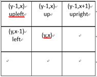
//计算四个方向邻域两像素的差别,也就是欧式距离或者说二阶范数
//(当所有像素都算完后,就相当于计算八邻域的像素差了)
Vec3d color = img.at(y,x);
if( x>0 ) // left >0的判断是为了避免在图像边界的时候还计算,导致越界
{
Vec3d diff = color - (Vec3d)img.at(y,x-1);
beta += diff.dot(diff); //矩阵的点乘,也就是各个元素平方的和
}
if( y>0 && x>0 ) // upleft
{
Vec3d diff = color - (Vec3d)img.at(y-1,x-1);
beta += diff.dot(diff);
}
if( y>0 ) // up
{
Vec3d diff = color - (Vec3d)img.at(y-1,x);
beta += diff.dot(diff);
}
if( y>0 && x(y-1,x+1);
beta += diff.dot(diff);
}
}
}
if( beta <= std::numeric_limits::epsilon() )
beta = 0;
else
beta = 1.f / (2 * beta/(4*img.cols*img.rows - 3*img.cols - 3*img.rows + 2) ); //论文公式(5)
return beta;
}
//计算图每个非端点顶点(也就是每个像素作为图的一个顶点,不包括源点s和汇点t)与邻域顶点
//的边的权值。由于是无向图,我们计算的是八邻域,那么对于一个顶点,我们计算四个方向就行,
//在其他的顶点计算的时候,会把剩余那四个方向的权值计算出来。这样整个图算完后,每个顶点
//与八邻域的顶点的边的权值就都计算出来了。
//这个相当于计算Gibbs能量的第二个能量项(平滑项),具体见论文中公式(4)
/*
Calculate weights of noterminal vertices of graph.
beta and gamma - parameters of GrabCut algorithm.
*/
static void calcNWeights( const Mat& img, Mat& leftW, Mat& upleftW, Mat& upW,
Mat& uprightW, double beta, double gamma )
{
//gammaDivSqrt2相当于公式(4)中的gamma * dis(i,j)^(-1),那么可以知道,
//当i和j是垂直或者水平关系时,dis(i,j)=1,当是对角关系时,dis(i,j)=sqrt(2.0f)。
//具体计算时,看下面就明白了
const double gammaDivSqrt2 = gamma / std::sqrt(2.0f);
//每个方向的边的权值通过一个和图大小相等的Mat来保存
leftW.create( img.rows, img.cols, CV_64FC1 );
upleftW.create( img.rows, img.cols, CV_64FC1 );
upW.create( img.rows, img.cols, CV_64FC1 );
uprightW.create( img.rows, img.cols, CV_64FC1 );
for( int y = 0; y < img.rows; y++ )
{
for( int x = 0; x < img.cols; x++ )
{
Vec3d color = img.at(y,x);
if( x-1>=0 ) // left //避免图的边界
{
Vec3d diff = color - (Vec3d)img.at(y,x-1);
leftW.at(y,x) = gamma * exp(-beta*diff.dot(diff));
}
else
leftW.at(y,x) = 0;
if( x-1>=0 && y-1>=0 ) // upleft
{
Vec3d diff = color - (Vec3d)img.at(y-1,x-1);
upleftW.at(y,x) = gammaDivSqrt2 * exp(-beta*diff.dot(diff));
}
else
upleftW.at(y,x) = 0;
if( y-1>=0 ) // up
{
Vec3d diff = color - (Vec3d)img.at(y-1,x);
upW.at(y,x) = gamma * exp(-beta*diff.dot(diff));
}
else
upW.at(y,x) = 0;
if( x+1=0 ) // upright
{
Vec3d diff = color - (Vec3d)img.at(y-1,x+1);
uprightW.at(y,x) = gammaDivSqrt2 * exp(-beta*diff.dot(diff));
}
else
uprightW.at(y,x) = 0;
}
}
}
//检查mask的正确性。mask为通过用户交互或者程序设定的,它是和图像大小一样的单通道灰度图,
//每个像素只能取GC_BGD or GC_FGD or GC_PR_BGD or GC_PR_FGD 四种枚举值,分别表示该像素
//(用户或者程序指定)属于背景、前景、可能为背景或者可能为前景像素。具体的参考:
//ICCV2001“Interactive Graph Cuts for Optimal Boundary & Region Segmentation of Objects in N-D Images”
//Yuri Y. Boykov Marie-Pierre Jolly
/*
Check size, type and element values of mask matrix.
*/
static void checkMask( const Mat& img, const Mat& mask )
{
if( mask.empty() )
CV_Error( CV_StsBadArg, "mask is empty" );
if( mask.type() != CV_8UC1 )
CV_Error( CV_StsBadArg, "mask must have CV_8UC1 type" );
if( mask.cols != img.cols || mask.rows != img.rows )
CV_Error( CV_StsBadArg, "mask must have as many rows and cols as img" );
for( int y = 0; y < mask.rows; y++ )
{
for( int x = 0; x < mask.cols; x++ )
{
uchar val = mask.at(y,x);
if( val!=GC_BGD && val!=GC_FGD && val!=GC_PR_BGD && val!=GC_PR_FGD )
CV_Error( CV_StsBadArg, "mask element value must be equel"
"GC_BGD or GC_FGD or GC_PR_BGD or GC_PR_FGD" );
}
}
}
//通过用户框选目标rect来创建mask,rect外的全部作为背景,设置为GC_BGD,
//rect内的设置为 GC_PR_FGD(可能为前景)
/*
Initialize mask using rectangular.
*/
static void initMaskWithRect( Mat& mask, Size imgSize, Rect rect )
{
mask.create( imgSize, CV_8UC1 );
mask.setTo( GC_BGD );
rect.x = max(0, rect.x);
rect.y = max(0, rect.y);
rect.width = min(rect.width, imgSize.width-rect.x);
rect.height = min(rect.height, imgSize.height-rect.y);
(mask(rect)).setTo( Scalar(GC_PR_FGD) );
}
//通过k-means算法来初始化背景GMM和前景GMM模型
/*
Initialize GMM background and foreground models using kmeans algorithm.
*/
static void initGMMs( const Mat& img, const Mat& mask, GMM& bgdGMM, GMM& fgdGMM )
{
const int kMeansItCount = 10; //迭代次数
const int kMeansType = KMEANS_PP_CENTERS; //Use kmeans++ center initialization by Arthur and Vassilvitskii
Mat bgdLabels, fgdLabels; //记录背景和前景的像素样本集中每个像素对应GMM的哪个高斯模型,论文中的kn
vector bgdSamples, fgdSamples; //背景和前景的像素样本集
Point p;
for( p.y = 0; p.y < img.rows; p.y++ )
{
for( p.x = 0; p.x < img.cols; p.x++ )
{
//mask中标记为GC_BGD和GC_PR_BGD的像素都作为背景的样本像素
if( mask.at(p) == GC_BGD || mask.at(p) == GC_PR_BGD )
bgdSamples.push_back( (Vec3f)img.at(p) );
else // GC_FGD | GC_PR_FGD
fgdSamples.push_back( (Vec3f)img.at(p) );
}
}
CV_Assert( !bgdSamples.empty() && !fgdSamples.empty() );
//kmeans中参数_bgdSamples为:每行一个样本
//kmeans的输出为bgdLabels,里面保存的是输入样本集中每一个样本对应的类标签(样本聚为componentsCount类后)
Mat _bgdSamples( (int)bgdSamples.size(), 3, CV_32FC1, &bgdSamples[0][0] );
kmeans( _bgdSamples, GMM::componentsCount, bgdLabels,
TermCriteria( CV_TERMCRIT_ITER, kMeansItCount, 0.0), 0, kMeansType );
Mat _fgdSamples( (int)fgdSamples.size(), 3, CV_32FC1, &fgdSamples[0][0] );
kmeans( _fgdSamples, GMM::componentsCount, fgdLabels,
TermCriteria( CV_TERMCRIT_ITER, kMeansItCount, 0.0), 0, kMeansType );
//经过上面的步骤后,每个像素所属的高斯模型就确定的了,那么就可以估计GMM中每个高斯模型的参数了。
bgdGMM.initLearning();
for( int i = 0; i < (int)bgdSamples.size(); i++ )
bgdGMM.addSample( bgdLabels.at(i,0), bgdSamples[i] );
bgdGMM.endLearning();//得到每个高斯模型的协方差逆矩阵,即计算inverseCovs[componentsCount][3][3]
fgdGMM.initLearning();
for( int i = 0; i < (int)fgdSamples.size(); i++ )
fgdGMM.addSample( fgdLabels.at(i,0), fgdSamples[i] );
fgdGMM.endLearning();
}
//论文中:迭代最小化算法step 1:为每个像素分配GMM中所属的高斯模型,kn保存在Mat compIdxs中
/*
Assign GMMs components for each pixel.
*/
static void assignGMMsComponents( const Mat& img, const Mat& mask, const GMM& bgdGMM,
const GMM& fgdGMM, Mat& compIdxs )
{
Point p;
for( p.y = 0; p.y < img.rows; p.y++ )
{
for( p.x = 0; p.x < img.cols; p.x++ )
{
Vec3d color = img.at(p);
//通过mask来判断该像素属于背景像素还是前景像素,再判断它属于前景或者背景GMM中的哪个高斯分量
compIdxs.at(p) = mask.at(p) == GC_BGD || mask.at(p) == GC_PR_BGD ?
bgdGMM.whichComponent(color) : fgdGMM.whichComponent(color);
}
}
}
//论文中:迭代最小化算法step 2:从每个高斯模型的像素样本集中学习每个高斯模型的参数
/*
Learn GMMs parameters.
*/
static void learnGMMs( const Mat& img, const Mat& mask, const Mat& compIdxs, GMM& bgdGMM, GMM& fgdGMM )
{
bgdGMM.initLearning();
fgdGMM.initLearning();
Point p;
for( int ci = 0; ci < GMM::componentsCount; ci++ )
{
for( p.y = 0; p.y < img.rows; p.y++ )
{
for( p.x = 0; p.x < img.cols; p.x++ )
{
if( compIdxs.at(p) == ci )
{
if( mask.at(p) == GC_BGD || mask.at(p) == GC_PR_BGD )
bgdGMM.addSample( ci, img.at(p) );
else
fgdGMM.addSample( ci, img.at(p) );
}
}
}
}
bgdGMM.endLearning();
fgdGMM.endLearning();
}
//通过计算得到的能量项构建图,图的顶点为像素点,图的边由两部分构成,
//一类边是:每个顶点与Sink汇点t(代表背景)和源点Source(代表前景)连接的边,
//这类边的权值通过Gibbs能量项的第一项能量项来表示。
//另一类边是:每个顶点与其邻域顶点连接的边,这类边的权值通过Gibbs能量项的第二项能量项来表示。
/*
Construct GCGraph
*/
static void constructGCGraph( const Mat& img, const Mat& mask, const GMM& bgdGMM, const GMM& fgdGMM, double lambda,
const Mat& leftW, const Mat& upleftW, const Mat& upW, const Mat& uprightW,
GCGraph& graph )
{
int vtxCount = img.cols*img.rows; //顶点数,每一个像素是一个顶点
int edgeCount = 2*(4*vtxCount - 3*(img.cols + img.rows) + 2); //边数,需要考虑图边界的边的缺失
//通过顶点数和边数创建图。这些类型声明和函数定义请参考gcgraph.hpp
graph.create(vtxCount, edgeCount);
Point p;
for( p.y = 0; p.y < img.rows; p.y++ )
{
for( p.x = 0; p.x < img.cols; p.x++)
{
// add node
int vtxIdx = graph.addVtx(); //返回这个顶点在图中的索引
Vec3b color = img.at(p);
// set t-weights
//计算每个顶点与Sink汇点t(代表背景)和源点Source(代表前景)连接的权值。
//也即计算Gibbs能量(每一个像素点作为背景像素或者前景像素)的第一个能量项
double fromSource, toSink;
if( mask.at(p) == GC_PR_BGD || mask.at(p) == GC_PR_FGD )
{
//对每一个像素计算其作为背景像素或者前景像素的第一个能量项,作为分别与t和s点的连接权值
fromSource = -log( bgdGMM(color) );
toSink = -log( fgdGMM(color) );
}
else if( mask.at(p) == GC_BGD )
{
//对于确定为背景的像素点,它与Source点(前景)的连接为0,与Sink点的连接为lambda
fromSource = 0;
toSink = lambda;
}
else // GC_FGD
{
fromSource = lambda;
toSink = 0;
}
//设置该顶点vtxIdx分别与Source点和Sink点的连接权值
graph.addTermWeights( vtxIdx, fromSource, toSink );
// set n-weights n-links
//计算两个邻域顶点之间连接的权值。
//也即计算Gibbs能量的第二个能量项(平滑项)
if( p.x>0 )
{
double w = leftW.at(p);
graph.addEdges( vtxIdx, vtxIdx-1, w, w );
}
if( p.x>0 && p.y>0 )
{
double w = upleftW.at(p);
graph.addEdges( vtxIdx, vtxIdx-img.cols-1, w, w );
}
if( p.y>0 )
{
double w = upW.at(p);
graph.addEdges( vtxIdx, vtxIdx-img.cols, w, w );
}
if( p.x0 )
{
double w = uprightW.at(p);
graph.addEdges( vtxIdx, vtxIdx-img.cols+1, w, w );
}
}
}
}
//论文中:迭代最小化算法step 3:分割估计:最小割或者最大流算法
/*
Estimate segmentation using MaxFlow algorithm
*/
static void estimateSegmentation( GCGraph& graph, Mat& mask )
{
//通过最大流算法确定图的最小割,也即完成图像的分割
graph.maxFlow();
Point p;
for( p.y = 0; p.y < mask.rows; p.y++ )
{
for( p.x = 0; p.x < mask.cols; p.x++ )
{
//通过图分割的结果来更新mask,即最后的图像分割结果。注意的是,永远都
//不会更新用户指定为背景或者前景的像素
if( mask.at(p) == GC_PR_BGD || mask.at(p) == GC_PR_FGD )
{
if( graph.inSourceSegment( p.y*mask.cols+p.x /*vertex index*/ ) )
mask.at(p) = GC_PR_FGD;
else
mask.at(p) = GC_PR_BGD;
}
}
}
}
//最后的成果:提供给外界使用的伟大的API:grabCut
/*
****参数说明:
img——待分割的源图像,必须是8位3通道(CV_8UC3)图像,在处理的过程中不会被修改;
mask——掩码图像,如果使用掩码进行初始化,那么mask保存初始化掩码信息;在执行分割
的时候,也可以将用户交互所设定的前景与背景保存到mask中,然后再传入grabCut函
数;在处理结束之后,mask中会保存结果。mask只能取以下四种值:
GCD_BGD(=0),背景;
GCD_FGD(=1),前景;
GCD_PR_BGD(=2),可能的背景;
GCD_PR_FGD(=3),可能的前景。
如果没有手工标记GCD_BGD或者GCD_FGD,那么结果只会有GCD_PR_BGD或GCD_PR_FGD;
rect——用于限定需要进行分割的图像范围,只有该矩形窗口内的图像部分才被处理;
bgdModel——背景模型,如果为null,函数内部会自动创建一个bgdModel;bgdModel必须是
单通道浮点型(CV_32FC1)图像,且行数只能为1,列数只能为13x5;
fgdModel——前景模型,如果为null,函数内部会自动创建一个fgdModel;fgdModel必须是
单通道浮点型(CV_32FC1)图像,且行数只能为1,列数只能为13x5;
iterCount——迭代次数,必须大于0;
mode——用于指示grabCut函数进行什么操作,可选的值有:
GC_INIT_WITH_RECT(=0),用矩形窗初始化GrabCut;
GC_INIT_WITH_MASK(=1),用掩码图像初始化GrabCut;
GC_EVAL(=2),执行分割。
*/
void cv::grabCut( InputArray _img, InputOutputArray _mask, Rect rect,
InputOutputArray _bgdModel, InputOutputArray _fgdModel,
int iterCount, int mode )
{
Mat img = _img.getMat();
Mat& mask = _mask.getMatRef();
Mat& bgdModel = _bgdModel.getMatRef();
Mat& fgdModel = _fgdModel.getMatRef();
if( img.empty() )
CV_Error( CV_StsBadArg, "image is empty" );
if( img.type() != CV_8UC3 )
CV_Error( CV_StsBadArg, "image mush have CV_8UC3 type" );
GMM bgdGMM( bgdModel ), fgdGMM( fgdModel );//初始化背景前景GMM模型bgdModel、fgdModel变成1*13的0向量。
Mat compIdxs( img.size(), CV_32SC1 );
if( mode == GC_INIT_WITH_RECT || mode == GC_INIT_WITH_MASK )
{
if( mode == GC_INIT_WITH_RECT )
initMaskWithRect( mask, img.size(), rect );//初始化mask,rect外面初始化为GCD_BGD,里面初始化为GCD_PR_FGD
else // flag == GC_INIT_WITH_MASK
checkMask( img, mask );
initGMMs( img, mask, bgdGMM, fgdGMM );
}
if( iterCount <= 0)
return;
if( mode == GC_EVAL )
checkMask( img, mask );
const double gamma = 50;//image是一个常量值50
const double lambda = 9*gamma;
const double beta = calcBeta( img );
Mat leftW, upleftW, upW, uprightW;
calcNWeights( img, leftW, upleftW, upW, uprightW, beta, gamma );
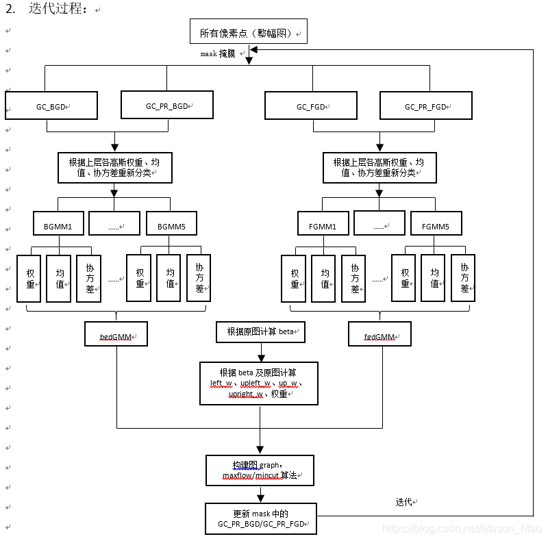
for( int i = 0; i < iterCount; i++ )
{
GCGraph graph;
assignGMMsComponents( img, mask, bgdGMM, fgdGMM, compIdxs );//通过mask来判断该像素属于背景像素还是前景像素,再判断它属于前景或者背景GMM中的哪个高斯分量
learnGMMs( img, mask, compIdxs, bgdGMM, fgdGMM );
constructGCGraph(img, mask, bgdGMM, fgdGMM, lambda, leftW, upleftW, upW, uprightW, graph );
estimateSegmentation( graph, mask );
}
}