自然语言处理 - LSA
LSA (Latent Semantic Analysis)潜在语义分析,是利用线性代数奇异值分解的方法来达到降维的目的。
有关奇异值分解,可以去参考线性代数的书籍。
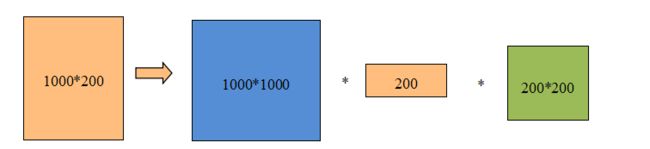
使用奇异值如何达到降维?正常的情况下,奇异值的分解并不能降低向量空间的复杂度。比如语料库是1000个单词,200篇文档的情况下,矩阵M的维度是1000x200,该矩阵有20万个元素。通过奇异值分解,可以得到三个矩阵,分别是1000x1000,200,200x200,一共有1,200,200个元素。可以发现经过奇异值分解后的维度增加了,而不是减少了。
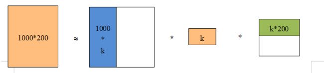
可以使用矩阵低秩近似的方法降低维度。首先将矩阵S中的n-k个最小的奇异值设为0,得到矩阵Sk(k要远远小于n)。再将矩阵U降维为Uk=m*k,矩阵V降维为Vk=k*n,令Mk=Uk*Sk*Vk,这样得到的矩阵就是矩阵M的低秩近似矩阵,并且低秩近似矩阵的维度远远低于M。
潜在语义分析(LSA)的原理以及实现方法如下:
(1)分析文档,建立词汇-文档矩阵
(2)对词汇-文档矩阵进行奇异值分解
(3)对奇异值分解后的矩阵进行降维
(4)使用降维后的矩阵构建潜在语义空间
下面通过一个具体的实例演示如何实现LSA。我们从网络是选取一些关于深度学习、神经网络以及语音识别的论文题目:
| 序号 | 文字名称 |
|---|---|
| 1 | Recurrent neural network based language model |
| 2 | Statistical Language Model Based on Neural Network |
| 3 | On the Importance of Initialization and Momentum in Deep Learning |
| 4 | A guide to recurrent neural network and backpropagation |
| 5 | Making Deep Belief Network Effective for Large Vocabulary Continuous Speech Recognition |
| 6 | Application Of Pretrained Deep Neural Network To Large Vocabulary Speech Recognition |
| 7 | Deep Neural Network for Acoustic Modeling in Speech Recognition |
| 8 | Flexible, High Performance Convolutional Neural Network for Image Classification |
| 9 | Best Practices for Convolutional Neural Network Applied to Visual Document Analysis |
| 10 | Deep Learning For Signal And Information Processing |
实现步骤如下:
(1)建立待分析的论文题目数组documents
(2)去掉一些不需要分析的词,比如:'for a of from on with in the and to’等
(3)构建字典对象,遍历所有的分词,统计每个分词出现的频率
(4)使用gensim的corpora生成字典。该字典包含有语料库里面出现频度大于1的词:
0 based
1 language
2 model
3 network
4 neural
5 recurrent
6 deep
7 learning
8 large
9 recognition
10 speech
11 vocabulary
12 convolutional
(5)使用gensim的词袋功能doc2word生成词频统计矩阵,矩阵如下:
[[(0, 1), (1, 1), (2, 1), (3, 1), (4, 1), (5, 1)],
 [(0, 1), (1, 1), (2, 1), (3, 1), (4, 1)],
 [(6, 1), (7, 1)],
 [(3, 1), (4, 1), (5, 1)],
 [(3, 1), (6, 1), (8, 1), (9, 1), (10, 1), (11, 1)],
 [(3, 1), (4, 1), (6, 1), (8, 1), (9, 1), (10, 1), (11, 1)],
 [(3, 1), (4, 1), (6, 1), (9, 1), (10, 1)],
 [(3, 1), (4, 1), (12, 1)],
 [(3, 1), (4, 1), (12, 1)],
 [(6, 1), (7, 1)]]
此矩阵由(词索引,频次)的二元数组组成。比如(0,1)表示索引为0的词(based)在第一个文章标题中出现了一次。(Recurrent neural network based language model)
(6)上面步骤生成的矩阵是无法直接给Numpy和Scipy使用的,需要使用共现矩阵。在共现矩阵中每一行代表一个词,而每一列是表示不同的上下文。矩阵中的元素表示相关词在上下文中出现的次数。
[[1., 1., 0., 0., 0., 0., 0., 0., 0., 0.],
       [1., 1., 0., 0., 0., 0., 0., 0., 0., 0.],
       [1., 1., 0., 0., 0., 0., 0., 0., 0., 0.],
       [1., 1., 0., 1., 1., 1., 1., 1., 1., 0.],
       [1., 1., 0., 1., 0., 1., 1., 1., 1., 0.],
       [1., 0., 0., 1., 0., 0., 0., 0., 0., 0.],
       [0., 0., 1., 0., 1., 1., 1., 0., 0., 1.],
       [0., 0., 1., 0., 0., 0., 0., 0., 0., 1.],
       [0., 0., 0., 0., 1., 1., 0., 0., 0., 0.],
       [0., 0., 0., 0., 1., 1., 1., 0., 0., 0.],
       [0., 0., 0., 0., 1., 1., 1., 0., 0., 0.],
       [0., 0., 0., 0., 1., 1., 0., 0., 0., 0.],
       [0., 0., 0., 0., 0., 0., 0., 1., 1., 0.]]
(7)使用Scipy的奇异值分解方法,分解这个二维矩阵,可以得到3个矩阵:
U:
[[-0.14, -0.3 , -0.37,  0.15,  0.23, -0.01,  0.06, -0.11,  0.81,  0.08, -0.02,  0.03, -0.08],
[ -0.14, -0.3 , -0.37,  0.15,  0.23, -0.01,  0.06, -0.11,  -0.34,  -0.74,  0.  , -0.  ,  0.01],
[-0.14, -0.3 , -0.37,  0.15,  0.23, -0.01,  0.06, -0.11,  -0.47,  0.66,  0.02,  -0.02,  0.06],
[-0.58, -0.16,  0.2 , -0.03, -0.02,  0.12,  0.38,  0.66,  0.  ,  0.  , -0.  ,  0.  , -0.  ],
       [-0.5 , -0.31,  0.24, -0.19, -0.1 , -0.25, -0.68, -0.16, -0.  ,    0.  ,  0.  , -0.  ,  0.  ],
       [-0.13, -0.23, -0.11,  0.02, -0.8 ,  0.31,  0.24, -0.35,  0.  , -0.  ,  0.  ,  0.  ,  0.  ],
       [-0.31,  0.44, -0.36, -0.4 , -0.01, -0.1 ,  0.08, -0.1 , -0.07,     0.02, -0.15,  0.2 , -0.58],
       [-0.03,  0.11, -0.38, -0.61,  0.02,  0.21, -0.09,  0.11,  0.07, -0.02,  0.15, -0.2 ,  0.58],
       [-0.19,  0.26, -0.01,  0.27,  0.09,  0.5 , -0.25, -0.03, -0.  , -0.  ,  0.06, -0.66, -0.24],
       [-0.28,  0.33,  0.02,  0.21, -0.02, -0.31,  0.17, -0.21,  0.03, -0.01, -0.61, -0.21,  0.43],
       [-0.28,  0.33,  0.02,  0.21, -0.02, -0.31,  0.17, -0.21,  0.03, -0.01,  0.76,  0.01,  0.15],
       [-0.19,  0.26, -0.01,  0.27,  0.09,  0.5 , -0.25, -0.03, -0.  , 0.  , -0.06,  0.66,  0.24],
       [-0.11, -0.12,  0.46, -0.34,  0.42,  0.28,  0.35, -0.52,  0.  , 0.  , -0.  , -0.  , -0.  ]]
S:
[[4.69, 0.  , 0.  , 0.  , 0.  , 0.  , 0.  , 0.  , 0.  , 0.  ],
       [0.  , 3.15, 0.  , 0.  , 0.  , 0.  , 0.  , 0.  , 0.  , 0.  ],
       [0.  , 0.  , 1.97, 0.  , 0.  , 0.  , 0.  , 0.  , 0.  , 0.  ],
       [0.  , 0.  , 0.  , 1.82, 0.  , 0.  , 0.  , 0.  , 0.  , 0.  ],
       [0.  , 0.  , 0.  , 0.  , 1.2 , 0.  , 0.  , 0.  , 0.  , 0.  ],
       [0.  , 0.  , 0.  , 0.  , 0.  , 1.03, 0.  , 0.  , 0.  , 0.  ],
       [0.  , 0.  , 0.  , 0.  , 0.  , 0.  , 0.54, 0.  , 0.  , 0.  ],
       [0.  , 0.  , 0.  , 0.  , 0.  , 0.  , 0.  , 0.31, 0.  , 0.  ],
       [0.  , 0.  , 0.  , 0.  , 0.  , 0.  , 0.  , 0.  , 0.  , 0.  ],
       [0.  , 0.  , 0.  , 0.  , 0.  , 0.  , 0.  , 0.  , 0.  , 0.  ]]
V:
[[-0.35, -0.32, -0.07, -0.26, -0.39, -0.49, -0.41, -0.25, -0.25, -0.07],
       [-0.5 , -0.43,  0.17, -0.22,  0.46,  0.36,  0.2 , -0.18, -0.18, 0.17],
       [-0.39, -0.33, -0.37,  0.17, -0.07,  0.05,  0.06,  0.46,  0.46, -0.37],
       [ 0.15,  0.13, -0.56, -0.11,  0.3 ,  0.19, -0.1 , -0.3 , -0.3 ,  -0.56],
       [-0.2 ,  0.47,  0.01, -0.76,  0.1 ,  0.02, -0.14,  0.25,  0.25, 0.01],
       [ 0.14, -0.15,  0.11,  0.17,  0.38,  0.14, -0.84,  0.14,  0.14,  0.11],
       [ 0.24, -0.21, -0.02, -0.11,  0.57, -0.7 ,  0.23,  0.09,  0.09,-0.02],
       [-0.58,  0.54,  0.02,  0.47,  0.26, -0.27, -0.05, -0.08, -0.08,  0.02],
       [-0.  , -0.  ,  0.71, -0.  , -0.  ,  0.  , -0.  ,  0.01, -0.01, -0.71],
       [-0.  , -0.  , -0.01,  0.  , -0.  ,  0.  ,  0.  ,  0.71, -0.71,   0.01]]
矩阵S就是奇异值。为了分析,取k=3,就是Sk 为:
[[4.69, 0.  , 0.  ]
[0. , 3.15, 0.  ]
[0. , 0.  , 1.97]]
对于的Uk,Vk.T也按此方法处理。
(8)分析
得到的UK是索引词的分布,Vk.T是文章题目的分布。这两个分布是3维的,观察3维空间难度比较大。可以只取两个维度,相当于投影到一个平面上。得到的结果如下图:
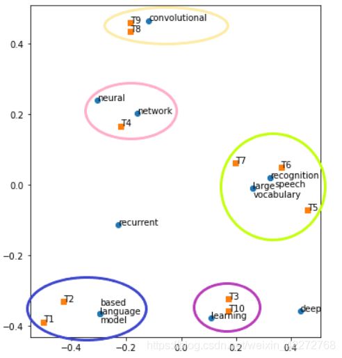
聚集在一起的索引词,可以解读为距离比较近,上下文的关联度比较强。而索引词与文章题目,可以当成摘要词。比如在最左下角的圆圈中,有文章标题T1和T2,而关键词有三个:based,language,model。这3个单词都也出现在了T1和T2中。
完成的代码如下:
from gensim import corpora, models, similarities
from collections import defaultdict
import numpy as np
import scipy
import matplotlib.pyplot as plt
import re


documents = [
'Recurrent neural network based language model',
'Statistical Language Model Based on Neural Network',
'On the Importance of Initialization and Momentum in Deep Learning',
'A guide to recurrent neural network and backpropagation',
'Making Deep Belief Network Effective for Large Vocabulary Continuous Speech Recognition',
'Application Of Pretrained Deep Neural Network To Large Vocabulary Speech Recognition',
'Deep Neural Network for Acoustic Modeling in Speech Recognition',
'Flexible, High Performance Convolutional Neural Network for Image Classification',
'Best Practices for Convolutional Neural Network Applied to Visual Document Analysis',
'Deep Learning For Signal And Information Processing'
    ]
#定义参数
n_novel=len(documents)
np.set_printoptions(precision=2, suppress=True)
n_pick_topics = 3           # 设定主题数为3

#去除常见虚拟词
stoplist=set('for a of from on with in the and to'.split())

def returnMatrix(array,size):
    length=len(array)
    M=np.zeros(shape=[size,length])
    i=0
    for index in array:
        for item in index:
            M[item[0],i]=item[1]
        i+=1
    return M
def SciPySVD(M):
    return  np.linalg.svd(M)

def DrowPic(u,vt,dict,n_novel):
    x=u[:,0]
    y=u[:,1]
    xv=vt[:,0]
    yv=vt[:,1]
    plt.scatter(x, y, marker='o')
    d=sorted(dict.keys())
    #y有重叠的标注,移动坐标以便清楚显示
    y[0]+=0.025
    y[2]-=0.025
    y[10]-=0.025
    x[10]+=0.015
    y[11]-=0.025
    yv[2]+=0.05
    yv[7]-=0.025
    yv[9]+=0.015
    #x[9]
    for i in d:
        plt.annotate(dict[i],xy=(x[i],y[i]))
    plt.scatter(xv,yv,marker='s')

    for i in range(n_novel):
        plt.annotate('T'+str(i+1),xy=(xv[i],yv[i]))


texts=[[word for word in document.lower().split() if word not in stoplist] for document in documents]
texts=[[re.sub('[’,:]+','',element) for element in item]for item in texts]

frequency = defaultdict(int) #构建一个字典对象
#遍历分词后的结果集,计算每个词出现的频率
for text in texts:
	for token in text:
		frequency[token]+=1
#选择频率大于1的词
texts=[[token for token in text if frequency[token]>1] for text in texts]

dictionary=corpora.Dictionary(texts)
import pprint as pp
for item in dictionary.items():
    print(item[0],item[1])
corpus = [dictionary.doc2bow(text) for text in texts]
pp.pprint(corpus)
M=returnMatrix(corpus,len(dictionary))
pp.pprint(M)
u,s,vt=SciPySVD(M)
pp.pprint(u)
pp.pprint(np.diag(s))
pp.pprint(vt)
DrowPic(u,vt.T,dictionary,n_novel)
plt.show()
以上的举例只是简要的说明了LSA的实现以及解释。LSA具有很多具有很多优势并被使用:
(1)LSA将文章和单词都映射到同一个语义空间,实现了文章聚类和单词聚类。通过聚类为结果可以基于单词的文献检索。
(2)LSA实现了降维,也同时降低了噪声的影响。
(3)LSA 是一个全局最优化算法,其目标是寻找全局最优解而非局部最优解。
LSA依然存在一些缺陷:
(1)首先LSA是假设服从高斯分布和2范数规范化的,因此它并非适合于所有场
(2)LSA不能有效处理一词多义问题。因为LSA的基本假设之一是单词只有一个词义。
(3)LSA的核心是SVD,而SVD的计算复杂度十分高并且难以更新新出现的文献。