field II 学习笔记1

calc_scat _all

目的： 计算从一组散射体接收到的信号的过程，以及计算孔径中每个传输和接收元件的组合的过程。这相当于一个全合成孔径扫描，每个元件发射，所有元件接收。请注意，原始数据是计算出来的。在数据上没有对焦或切趾，这必须在之后的数据上进行。一个32元件的传感器会有1024个信号。
调用：

[scat, start time] = calc_scat_all (Th1, Th2, points, amplitudes, dec factor);

参数：

输入	解释
Th1	指向发射孔径的指针
Th2	指向发射孔径的指针
points	散射点。三列向量（x,y,z），每一行代表一个散射点
dec_factor	输出采样率的抽取因子。采样频率就是$\frac{fs}{dec\_factor}$
amplitudes	散射振幅。行向量，元素代表每个散射点振幅

输出	解释
scat	接收电压，矩阵每个元素是一个接收单元的一个接收信号，第一个信号是单元1接收到单元1发送的信号
start_time	scat中第一个样本的时间

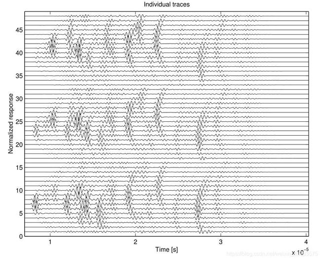
示例： 计算由3个发射单元和16个接收单元组成的线性阵列的所有单元的接收响应，并绘制响应和总响应。

clear,close all, clc,
field_init;
%  Set initial parameters
f0=3e6; %  Transducer center frequency [Hz]
fs=100e6; %  Sampling frequency [Hz]
c=1540; %  Speed of sound [m/s]
lambda=c/f0; %  Wavelength [m]
height=5/1000; %  Height of element [m]
width=1/1000; %  Width of element [m]
kerf=width/5; %  Distance between transducer elements [m]
N_elements=3; %  Number of elements
N_elements2=16; %  Number of elements
focus=[0 0 40]/1000;  %  Initial electronic focus
%  Define the transducers
Th = xdc_linear_array (N_elements, width, height, kerf, 2, 3, focus);
Th2 = xdc_linear_array (N_elements2, width, height, kerf, 2, 3, focus);
%  Set the impulse response and excitation of the emit aperture
impulse_response=sin(2*pi*f0*(0:1/fs:2/f0));
impulse_response=impulse_response.*hanning(max(size(impulse_response)))';
xdc_impulse (Th, impulse_response);
xdc_impulse (Th2, impulse_response);
excitation=sin(2*pi*f0*(0:1/fs:2/f0));
xdc_excitation (Th, excitation);
%  Define a small phantom with scatterers
N=200; %  Number of scatterers
x_size = 20/1000;  %  Width of phantom [mm]
y_size = 10/1000;  %  Transverse width of phantom [mm]
z_size = 20/1000;  %  Height of phantom [mm]
z_start = 5/1000;  %  Start of phantom surface [mm];
%  Create the general scatterers
x = (rand (N,1)-0.5)*x_size;
y = (rand (N,1)-0.5)*y_size;
z = rand (N,1)*z_size + z_start;
positions=[x y z];
%  Generate the amplitudes with a Gaussian distribution
amp=randn(N,1);
%  Do the calculation
[v,t]=calc_scat_all (Th, Th2, positions, amp, 1);
%  Plot the individual responses
[N,M]=size(v);
scale=max(max(v));
v=v/scale;
for i=1:M
plot((0:N-1)/fs+t,v(:,i)+i,'b'), hold on
end
hold off
title('Individual traces')
xlabel('Time [s]')
ylabel('Normalized response')
axis([t t+N/fs 0 M+1])

xdc_linear_array

目的：

调用：

Th = xdc_linear_array (no_elements, width, height, kerf, no_sub_x, no_sub_y, focus);

参数：

输入	解释
no_elements	物理阵元的数量
width	阵元x方向的宽度
height	阵元y方向的宽度
kerf	阵元之间x方向的距离
no_sub_x	阵元x方向子划分数
no_sub_y	阵元y方向子划分数
focus[]	固定焦点(x,y,z)

输出	解释
Th	该传感器孔径指针

示例略