深度学习二分类问题--IMDB数据集

环境使用keras为前端，TensorFlow为后端

 

IMDB数据集包含50000条评论，25000条用于训练，25000条用于测试，训练集和测试集都包含了50%的正面评论和负面评论

首先是加载IMDB数据集：

from keras.datasets import imdb

(train_data, train_labels), (test_data, test_labels) = imdb.load_data(num_words=10000)

num_words=10000表示保留训练数据中前10000个最常出现的单词。

train_data和test_data这两个变量都是评论组成的列表，每条评论又是单词索引组成的列表。train_labels和test_labels都是0和1组成的列表，0为负面评论，1为正面评论。

如果想要将某条评论迅速解码为英文单词，代码如下

#word_index是一个将单词映射为整数索引的字典
word_index = imdb.get_word_index()
#键值颠倒。将整数索引映射为单词
reverse_word_index = dict([(value, key) for (key, value) in word_index.items()])
#将评论解码。索引之所以-3是因为0,1,2是'padding'，'start of sequence','unknown'分别保留的索引
decoded_review = ' '.join([reverse_word_index.get(i - 3, '?') for i in train_data[0]])
decoded_review

结果如下：

"? this film was just brilliant casting location scenery story direction everyone's 
really suited the part they played and you could just imagine being there robert ? is an 
amazing actor and now the same being director ? father came from the same scottish 
island as myself so i loved the fact there was a real connection with this film the 
witty remarks throughout the film were great it was just brilliant so much that i bought 
the film as soon as it was released for ? and would recommend it to everyone to watch 
and the fly fishing was amazing really cried at the end it was so sad and you know what 
they say if you cry at a film it must have been good and this definitely was also ? to 
the two little boy's that played the ? of norman and paul they were just brilliant 
children are often left out of the ? list i think because the stars that play them all 
grown up are such a big profile for the whole film but these children are amazing and 
should be praised for what they have done don't you think the whole story was so lovely 
because it was true and was someone's life after all that was shared with us all"

准备数据：

首先要明白整数序列是不能直接输入神经网络的，所以要先将列表转换为张量，有两种方法，分别为填充列表和对列表进行one_hot编码。代码如下，下列代码采用的是one_hot编码。

import numpy as np

def vectorize_sequences(sequences, dimension=10000):
    # 创建一个形状为(len(sequences), dimension)的零矩阵
    results = np.zeros((len(sequences), dimension))
    for i, sequence in enumerate(sequences):
        #sequence中的值对应的列向量为1,如i为0，sequence中有值为1，则results第0行第1列为1
        results[i,sequence] = 1.  # set specific indices of results[i] to 1s
    return results

#将训练数据向量化
x_train = vectorize_sequences(train_data)
#将测试数据向量化
x_test = vectorize_sequences(test_data)

#标签向量化，并不像数据的向量化那样麻烦，因为本身就是值为0,1的一维列表，直接转换即可
y_train = np.asarray(train_labels).astype('float32')
y_test = np.asarray(test_labels).astype('float32')

如下方所示，为第0行的0-99列的one_hot编码

(x_train[0][0:100])

array([0., 1., 1., 0., 1., 1., 1., 1., 1., 1., 0., 0., 1., 1., 1., 1., 1.,
       1., 1., 1., 0., 1., 1., 0., 0., 1., 1., 0., 1., 0., 1., 0., 1., 1.,
       0., 1., 1., 0., 1., 1., 0., 0., 0., 1., 0., 0., 1., 0., 1., 0., 1.,
       1., 1., 0., 0., 0., 1., 0., 0., 0., 0., 0., 1., 0., 0., 1., 1., 0.,
       0., 0., 0., 1., 0., 0., 0., 0., 1., 1., 0., 0., 0., 0., 1., 0., 0.,
       0., 0., 1., 1., 0., 0., 0., 1., 0., 0., 0., 0., 0., 1., 0.])

构建网络

from keras import models
from keras import layers
#Sequential模型是多个网络层的线性堆叠，是函数式模型的一种特殊情况，functional的类名为model
model = models.Sequential()
#向模型中加入一个全连接层，16为该层隐藏单元的个数，一个隐藏单元是该层表示空间的一个维度，每个带relu激活的Dence层(全连接层)都实现了以下张量运算：output=relu(dot(w,input)+b)。16个隐藏单元对应的权重矩阵W的形状为(nput_dimension,16),与w做点积相当于将输入数据投影到16维表示空间中。
model.add(layers.Dense(16, activation='relu', input_shape=(10000,)))
model.add(layers.Dense(16, activation='relu'))
#最后一层使用sigmoid函数输出一个0-1的概率值，relu函数将所有的负值归0.sigmoid函数将人一直压缩到0-1的区间内
model.add(layers.Dense(1, activation='sigmoid'))

选择损失函数和优化器，此问题为二分类问题，输出是一个概率值，那么使用binary_crossentropy(二元交叉熵)损失。，对于输出概率值的模型，交叉熵往往是最好的选择。

下面为用rmsprop优化器和binary_crossentropy损失函数来配置模型

model.compile(optimizer='rmsprop',loss='binary_crossentropy',metrics=['accuracy'])

为了监控训练过程中在未曾见过的数据上的精度，将原始数据留出10000个样本作为验证集

x_val = x_train[:10000]
partial_x_train = x_train[10000:]

y_val = y_train[:10000]
partial_y_train = y_train[10000:]

现使用512个样本组成的小批量数据，将模型训练20个轮次（即对x_train和y_train两个张量中的所有样本进行20次迭代）。同时，为了监控留出的10000个样本上的损失和精度，将验证数据传入validation_data参数来完成

history = model.fit(partial_x_train,
                    partial_y_train,
                    epochs=20,
                    batch_size=512,
                    validation_data=(x_val, y_val))

调用model.fit()返回了一个histroy对象，这个对象有一个成员histroy，为一个字典，包含训练过程中的所有数据。

绘制训练损失和验证损失由于随机初始化不同，得到的结果并不一定相同

import matplotlib.pyplot as plt

acc = history.history['acc']
val_acc = history.history['val_acc']
loss = history.history['loss']
val_loss = history.history['val_loss']

epochs = range(1, len(loss) + 1)

# "bo" is for "blue dot"
plt.plot(epochs, loss, 'bo', label='Training loss')
# b is for "solid blue line"
plt.plot(epochs, val_loss, 'b', label='Validation loss')
plt.title('Training and validation loss')
plt.xlabel('Epochs')
plt.ylabel('Loss')
plt.legend()

plt.show()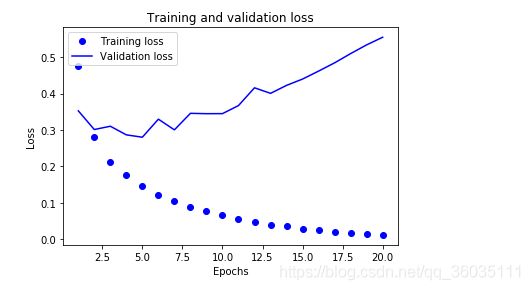

plt.clf()   # clear figure
acc_values = history_dict['acc']
val_acc_values = history_dict['val_acc']

plt.plot(epochs, acc, 'bo', label='Training acc')
plt.plot(epochs, val_acc, 'b', label='Validation acc')
plt.title('Training and validation accuracy')
plt.xlabel('Epochs')
plt.ylabel('Loss')
plt.legend()

plt.show()

 

 

由图可见，训练损失每轮都在降低，训练精度每轮都在提升。但验证损失和验证精度并非如此。

最后就可以使用predict方法得到评论为正面的可能性大小

model.predict(x_test)
#如前10个数据
array([[0.13560075],
       [0.9997118 ],
       [0.27816266],
       [0.6444917 ],
       [0.9250585 ],
       [0.67139983],
       [0.998109  ],
       [0.00650506],
       [0.9360959 ],
       [0.9851424 ]], dtype=float32)
#对应的labels标签
array([0, 1, 1, 0, 1, 1, 1, 0, 0, 1])
array([[0.02645707],
       [0.00111707],
       [0.2659221 ],
       [0.09683183],
       [0.00263329],
       [0.01840624],
       [0.99065304],
       [0.35139275],
       [0.9867306 ],
       [0.02706625]], dtype=float32)
对应的labels标签
array([1, 0, 0, 0, 0, 0, 1, 1, 1, 0])

可以发现验证精度并不够高，这是因为发生了过拟合。而且网络对某些样本非常确信(0.99,0.01)但有些结果却不太确信(0.4,0.6)