matplotlib 配色之内置 colormap

Matplotlib 配色之内置 colormap

概述

让图表看起来比较美观是图表配色最末的目的，配色最核心的目标是为你的数据集找到一个好的表达。

对于任何给定的数据集，最佳的配色取决于许多因素，包括:

• 表现形式或者度量数据。
• 你对数据集的理解（如：是否有一个偏离其它值的临界值？）
• 如果你正在绘制的参数（变量本身）有一个直观的配色方案
• 如果在这个领域有一个标准（行业配色标准或习惯），读者可能会期待

对于许多应用程序，感知上一致的配色是最佳选择。如，数据中的相同步幅被视为颜色空间中的相同步幅（色彩间的变化反映了数据的变化）。

感知是观众对不同颜色、或不同颜色组合的情感反应。

matplotlib提供了三个模块用于对图表的颜色进行操控：

1. matplotlib.cm
2. matplotlib.colorbar
3. matplotlib.colors

在matplotlib中，有三种给图表配色的方法：

1. 直观的指定颜色，如，在对象的参数中指定,color='red'；
2. 使用colormap，将数据映射为颜色模型。注意，需要支持 cmap 参数的图表类型；
3. 通过y值，使用蒙版数组按y值绘制具有不同颜色的线。

前面的文章已详细介绍了 方法1、2，下面用一个示例介绍方法3。

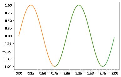
使用masked arrays组线条着不同的颜色

%matplotlib inline
import numpy as np
import matplotlib.pyplot as plt

t = np.arange(0.0, 2.0, 0.01)
s = np.sin(2 * np.pi * t)

upper = 0.77
lower = -0.77

supper = np.ma.masked_where(s < upper, s)
slower = np.ma.masked_where(s > lower, s)
smiddle = np.ma.masked_where((s < lower) | (s > upper), s)

fig, ax = plt.subplots()
ax.plot(t, smiddle, t, slower, t, supper)
plt.show()

%matplotlib inline
import numpy as np
import matplotlib.pyplot as plt

t = np.arange(0.0, 2.0, 0.01)
s = np.sin(2 * np.pi * t)

upper =0.75
lower = 1.75

supper = np.ma.masked_where(t < upper, s)
slower = np.ma.masked_where(t > lower, s)
smiddle = np.ma.masked_where((t < lower) | (t > upper), t)

fig, ax = plt.subplots()
ax.plot(t, smiddle, t, slower, t, supper)
plt.show()

matplotlib内置的colormap

matplotlib内置了7类colormap，用于不同的场景：

1. Perceptually Uniform Sequential
2. Sequential
3. Sequential2
4. Diverging
5. Cyclic
6. Qualitative
7. Miscellaneous

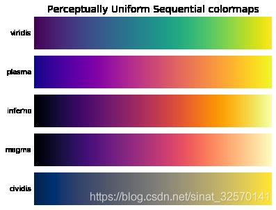
Perceptually Uniform Sequential

Sequential，顺序排列的，连续、有序的。

明度、亮度的变化，通常是颜色的饱和度逐渐增加，经常使用单一的色相；适合用于表示具有顺序的信息。

"Perceptually Uniform Sequential"类colormap提供了5种数值到颜色的映射序列，左边是亮度较低（亮度较暗的色相），右边则是较亮的色相。

cmaps['Perceptually Uniform Sequential'] = [
            'viridis', 'plasma', 'inferno', 'magma', 'cividis']

from colorspacious import cspace_convert

# sphinx_gallery_thumbnail_number = 2

import numpy as np
import matplotlib as mpl
import matplotlib.pyplot as plt
from matplotlib import cm
from colorspacious import cspace_converter
from collections import OrderedDict

cmaps = OrderedDict()

cmaps['Perceptually Uniform Sequential'] = [
            'viridis', 'plasma', 'inferno', 'magma', 'cividis']

nrows = max(len(cmap_list) for cmap_category, cmap_list in cmaps.items())
gradient = np.linspace(0, 1, 256)
gradient = np.vstack((gradient, gradient))

def plot_color_gradients(cmap_category, cmap_list, nrows):
    fig, axes = plt.subplots(nrows=nrows)
    fig.subplots_adjust(top=0.95, bottom=0.01, left=0.2, right=0.99)
    axes[0].set_title(cmap_category + ' colormaps', fontsize=14)

    for ax, name in zip(axes, cmap_list):
        ax.imshow(gradient, aspect='auto', cmap=plt.get_cmap(name))
        pos = list(ax.get_position().bounds)
        x_text = pos[0] - 0.01
        y_text = pos[1] + pos[3]/2.
        fig.text(x_text, y_text, name, va='center', ha='right', fontsize=10)

    # Turn off *all* ticks & spines, not just the ones with colormaps.
    for ax in axes:
        ax.set_axis_off()


for cmap_category, cmap_list in cmaps.items():
    plot_color_gradients(cmap_category, cmap_list, nrows)

plt.show()

print(cmaps)

OrderedDict([('Perceptually Uniform Sequential', ['viridis', 'plasma', 'inferno', 'magma', 'cividis'])])

获取colormap颜色信息

以RGB颜色为例，colormap每个映射使用一个(256,3)，即256行，3列的array存储颜色信息。每行代表colormap映射条上的一个点。

可以使用下面的代码读取cmp的颜色信息：

#读取cmp单个点的颜色的RGB值

from matplotlib import cm

def get_pcv(cn,r):
    #cn是cmap实例，例如 cn = cm.viridis, cm=cm.jet
    #r是行号，整数，如12
   
    print(cn(r)[0],cn(r)[1],cn(r)[2])
    #转换为256色表示的整数
    print(int(cn(r)[0]*255.0),int(cn(r)[1]*255.0),int(cn(r)[2]*255.0)) 

piyg_l = [x for x in cm.PiYG._segmentdata['green']]

def prc(cmap):
    for y in cmap:
        for l in y:
            print(l*255)

prc(piyg_l)

#print(len(piyg_l))

#print(piyg_l)

0.0
1.0
1.0
25.5
27.0
27.0
51.0
119.0
119.0
76.50000000000001
182.0
182.0
102.0
224.0
224.0
127.5
247.0
247.0
153.00000000000003
245.0
245.0
178.50000000000003
225.0
225.0
204.0
188.0
188.0
229.5
146.0
146.0
255.0
100.0
100.0

bwr_l = [x*255 for x in cm.bwr._segmentdata['green'][2]]

print(len(bwr_l))

print(bwr_l)

3
[255.0, 0.0, 0.0]

get_pcv(cm.viridis,0)

0.267004 0.004874 0.329415
68 1 84

每个colormap实例都有一个name属性，返回映射的名称。

from matplotlib import cm

cn = cm.viridis

cn.name

'viridis'

获取colormap实例的映射值

如此众多的colormaps，使用下面的代码，可以将这些colormap中具体的数值导出来，以供更深入地研究、更灵活地使用。

#获取colormap实例的映射值

from matplotlib import cm
 
def get_cmv(cn):
    #cn是colormap的实例，如cm.viridis, cm.jet等
 
    import numpy as np
    
    #创建全部为0的(256,3)的数组
    colormap_int = np.zeros((256, 3), np.uint8)
    colormap_float = np.zeros((256, 3), np.float)
    
    #将每个点值读取，存入上面的数组
 
    for i in range(0, 256, 1):
       colormap_float[i, 0] = cn(i)[0]
       colormap_float[i, 1] = cn(i)[1]
       colormap_float[i, 2] = cn(i)[2]
 
       colormap_int[i, 0] = np.int_(np.round(cn(i)[0] * 255.0))
       colormap_int[i, 1] = np.int_(np.round(cn(i)[1] * 255.0))
       colormap_int[i, 2] = np.int_(np.round(cn(i)[2] * 255.0))
    
    #将数组保存到txt文件 
    np.savetxt(str(cn.name)+"_float.txt", colormap_float, fmt = "%f", delimiter = ' ', newline = '\n')
    np.savetxt(str(cn.name)+"_int.txt", colormap_int, fmt = "%d", delimiter = ' ', newline = '\n')
    
    #打印相关信息 
    #print(colormap_int)
    print(colormap_int.shape)
    print(colormap_int)
 
    return

#调用get_cmv()函数，提供colormap实例作为参数

get_cmv(cm.viridis)

(256, 3)
[[ 68   1  84]
 [ 68   2  86]
 [ 69   4  87]
 [ 69   5  89]
 [ 70   7  90]
 [ 70   8  92]
 [ 70  10  93]
 [ 70  11  94]
 [ 71  13  96]
 [ 71  14  97]
 [ 71  16  99]
 [ 71  17 100]
 [ 71  19 101]
 [ 72  20 103]
 [ 72  22 104]
 [ 72  23 105]
 [ 72  24 106]
 [ 72  26 108]
 [ 72  27 109]
 [ 72  28 110]
 [ 72  29 111]
 [ 72  31 112]
 [ 72  32 113]
 [ 72  33 115]
 [ 72  35 116]
 [ 72  36 117]

…

Sequential,

对于序列图，亮度值通过颜色图单调增加。

colormaps中的一些 $L^{\ast }$ 值（亮度值）的范围是从0到100（二进制和其他灰度级），其他的在 $L^{\ast }=20$ 左右开始。 $L^{\ast }$ 函数在colormap之间是不同的：有些在 $L^{\ast }$ 中是近线性的，而其他的则是较为弯曲的。

Sequential类colormap有如下特性：

• 通常是单一色相的亮度变化；
• 亮度值变化范围从0到100；
• 有些是线性变化的，有些则是曲线的；
• 同一色相有亮度变化，不同色相之间的亮度不同。

# sphinx_gallery_thumbnail_number = 2

import numpy as np
import matplotlib as mpl
import matplotlib.pyplot as plt
from matplotlib import cm
from colorspacious import cspace_converter
from collections import OrderedDict

cmaps = OrderedDict()

cmaps['Sequential'] = [
            'Greys', 'Purples', 'Blues', 'Greens', 'Oranges', 'Reds',
            'YlOrBr', 'YlOrRd', 'OrRd', 'PuRd', 'RdPu', 'BuPu',
            'GnBu', 'PuBu', 'YlGnBu', 'PuBuGn', 'BuGn', 'YlGn']

nrows = max(len(cmap_list) for cmap_category, cmap_list in cmaps.items())
gradient = np.linspace(0, 1, 256)
gradient = np.vstack((gradient, gradient))

for cmap_category, cmap_list in cmaps.items():
    plot_color_gradients(cmap_category, cmap_list, nrows)

plt.show()

print(cmaps)

OrderedDict([('Sequential', ['Greys', 'Purples', 'Blues', 'Greens', 'Oranges', 'Reds', 'YlOrBr', 'YlOrRd', 'OrRd', 'PuRd', 'RdPu', 'BuPu', 'GnBu', 'PuBu', 'YlGnBu', 'PuBuGn', 'BuGn', 'YlGn'])])

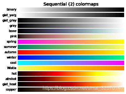
Sequential2

Sequential2类别中许多颜色映射模型的 $L^{\ast }$ 值都是单调增加的，但是某些映射模型 (autumn, cool, spring, and winter) 在$L^{\ast }$ 空间中达到平稳，或者甚至上下波动。其它映射模型(afmhot, copper, gist_heat, and hot) 在 $L^{\ast }$ 函数中有纽结。在平稳或扭结的colormap区域中表示的数据将在colormap的这些值处导致数据条带的感觉。

# sphinx_gallery_thumbnail_number = 2

import numpy as np
import matplotlib as mpl
import matplotlib.pyplot as plt
from matplotlib import cm
from colorspacious import cspace_converter
from collections import OrderedDict

cmaps = OrderedDict()

cmaps['Sequential (2)'] = [
            'binary', 'gist_yarg', 'gist_gray', 'gray', 'bone', 'pink',
            'spring', 'summer', 'autumn', 'winter', 'cool', 'Wistia',
            'hot', 'afmhot', 'gist_heat', 'copper']

nrows = max(len(cmap_list) for cmap_category, cmap_list in cmaps.items())
gradient = np.linspace(0, 1, 256)
gradient = np.vstack((gradient, gradient))

for cmap_category, cmap_list in cmaps.items():
    plot_color_gradients(cmap_category, cmap_list, nrows)

plt.show()

print(cmaps)

OrderedDict([('Sequential (2)', ['binary', 'gist_yarg', 'gist_gray', 'gray', 'bone', 'pink', 'spring', 'summer', 'autumn', 'winter', 'cool', 'Wistia', 'hot', 'afmhot', 'gist_heat', 'copper'])])

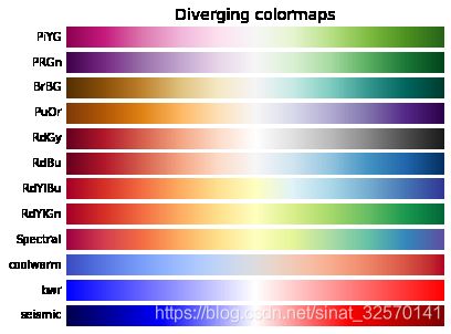
Diverging 发散

对于 Diverging 映射，我们希望 $L^{\ast }$ 值单调增加到最大值，该值应接近 $L^{\ast }=100$, 然后单调减小 $L^{\ast }$ 值。我们在colormap的相对两端寻找近似相等的最小 $L^{\ast }$ 值。通过这些措施，BrBG and RdBu 是不错的选择。coolwarm 是一个不错的选择，但它不能涵盖范围广泛的 $L^{\ast }$ 值 。

# sphinx_gallery_thumbnail_number = 2

import numpy as np
import matplotlib as mpl
import matplotlib.pyplot as plt
from matplotlib import cm
from colorspacious import cspace_converter
from collections import OrderedDict

cmaps = OrderedDict()

cmaps['Diverging'] = [
            'PiYG', 'PRGn', 'BrBG', 'PuOr', 'RdGy', 'RdBu',
            'RdYlBu', 'RdYlGn', 'Spectral', 'coolwarm', 'bwr', 'seismic']

nrows = max(len(cmap_list) for cmap_category, cmap_list in cmaps.items())
gradient = np.linspace(0, 1, 256)
gradient = np.vstack((gradient, gradient))

for cmap_category, cmap_list in cmaps.items():
    plot_color_gradients(cmap_category, cmap_list, nrows)

plt.show()

print(cmaps)

OrderedDict([('Diverging', ['PiYG', 'PRGn', 'BrBG', 'PuOr', 'RdGy', 'RdBu', 'RdYlBu', 'RdYlGn', 'Spectral', 'coolwarm', 'bwr', 'seismic'])])

Cyclic 循环的

对于循环的映射，我们希望以相同的颜色开始和结束，并在中间遇到一个对称的中心点。$L^{\ast }$ 应该从开始到中间单调变化，再从中间到结尾反向单调变化。它在增加和减少方面应该是对称的，并且只有色相不同。在两端和中间，$L^{\ast }$ 将反转方向，应在 $L^{\ast }$ 区间中进行平滑处理以减少伪像。

尽管此HSV颜色映射与中心点不对称，但它仍包含在这组颜色映射中。此外， $L^{\ast }$ 值在整个颜色映射中变化很大，因此对于表示供观看者感知的数据而言，这是一个糟糕的选择。请在 mycarta-jet上查看有关此想法的扩展。

# sphinx_gallery_thumbnail_number = 2

import numpy as np
import matplotlib as mpl
import matplotlib.pyplot as plt
from matplotlib import cm
from colorspacious import cspace_converter
from collections import OrderedDict

cmaps = OrderedDict()

cmaps['Cyclic'] = ['twilight', 'twilight_shifted', 'hsv']

nrows = max(len(cmap_list) for cmap_category, cmap_list in cmaps.items())
gradient = np.linspace(0, 1, 256)
gradient = np.vstack((gradient, gradient))

for cmap_category, cmap_list in cmaps.items():
    plot_color_gradients(cmap_category, cmap_list, nrows)

plt.show()

print(cmaps)

OrderedDict([('Cyclic', ['twilight', 'twilight_shifted', 'hsv'])])

Qualitative 定性

定性的 colormaps $L^{\ast }$ 值在colormap上四处移动，显然不是单调递增的。

# sphinx_gallery_thumbnail_number = 2

import numpy as np
import matplotlib as mpl
import matplotlib.pyplot as plt
from matplotlib import cm
from colorspacious import cspace_converter
from collections import OrderedDict

cmaps = OrderedDict()

cmaps['Qualitative'] = ['Pastel1', 'Pastel2', 'Paired', 'Accent',
                        'Dark2', 'Set1', 'Set2', 'Set3',
                        'tab10', 'tab20', 'tab20b', 'tab20c']

nrows = max(len(cmap_list) for cmap_category, cmap_list in cmaps.items())
gradient = np.linspace(0, 1, 256)
gradient = np.vstack((gradient, gradient))

for cmap_category, cmap_list in cmaps.items():
    plot_color_gradients(cmap_category, cmap_list, nrows)

plt.show()

print(cmaps)

OrderedDict([('Qualitative', ['Pastel1', 'Pastel2', 'Paired', 'Accent', 'Dark2', 'Set1', 'Set2', 'Set3', 'tab10', 'tab20', 'tab20b', 'tab20c'])])

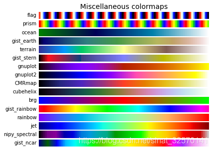
Miscellaneous 杂项

一些杂项 colormaps 有其特定用途。例如，gist_earth, ocean, and terrain 似乎都是为一起绘制地形 topography (green/brown) 和水深 (blue) 而创建的。我们期望在这些 colormaps 看到一个（气流或海洋的）分开处, 然而，但是在gist_earth和地形中，多种扭结可能不是最理想的。创建CMRmap是为了很好地转换为灰度。尽管它在$L^{\ast }$中似乎存在一些小问题。立方体螺旋被创造在亮度和色调上平滑地变化，但是在绿色色调区域似乎有一个小隆起。

常用的jet colormap包含在这组colormap中。我们可以看到，$L^{\ast }$值在整个colormap中变化很大，这使得它成为一个糟糕的选择，不能代表查看者能够感知到的数据。在mycarta-jet可以看到这个想法的扩展。

# sphinx_gallery_thumbnail_number = 2

import numpy as np
import matplotlib as mpl
import matplotlib.pyplot as plt
from matplotlib import cm
from colorspacious import cspace_converter
from collections import OrderedDict

cmaps = OrderedDict()

cmaps['Miscellaneous'] = [
            'flag', 'prism', 'ocean', 'gist_earth', 'terrain', 'gist_stern',
            'gnuplot', 'gnuplot2', 'CMRmap', 'cubehelix', 'brg',
            'gist_rainbow', 'rainbow', 'jet', 'nipy_spectral', 'gist_ncar']

nrows = max(len(cmap_list) for cmap_category, cmap_list in cmaps.items())
gradient = np.linspace(0, 1, 256)
gradient = np.vstack((gradient, gradient))

for cmap_category, cmap_list in cmaps.items():
    plot_color_gradients(cmap_category, cmap_list, nrows)

plt.show()

print(cmaps)

OrderedDict([('Miscellaneous', ['flag', 'prism', 'ocean', 'gist_earth', 'terrain', 'gist_stern', 'gnuplot', 'gnuplot2', 'CMRmap', 'cubehelix', 'brg', 'gist_rainbow', 'rainbow', 'jet', 'nipy_spectral', 'gist_ncar'])])

colormap可用的映射名称

内置的映射名称

matplotlib内置了7类，82种颜色映射，每种颜色映射又有一个反向映射，共164种。

当使用cm.get_cmap(name)方法返回内置的colormap实例时，如果name参数不在内置的映射中，就会触发如下错误，并提示可用的名称：

ValueError: Colormap NoNmae is not recognized. Possible values are: 

下面的代码就会触发上述错误：

%matplotlib inline

import matplotlib as mpl

cmap = mpl.cm.get_cmap('noname')

可用的名称值有:

1	2	3	4	5	6
Accent	Accent_r	Blues	Blues_r	BrBG	BrBG_r
BuGn	BuGn_r	BuPu	BuPu_r	CMRmap	CMRmap_r
Dark2	Dark2_r	GnBu	GnBu_r	Greens	Greens_r
Greys	Greys_r	OrRd	OrRd_r	Oranges	Oranges_r
PRGn	PRGn_r	Paired	Paired_r	Pastel1	Pastel1_r
Pastel2	Pastel2_r	PiYG	PiYG_r	PuBu	PuBuGn
PuBuGn_r	PuBu_r	PuOr	PuOr_r	PuRd	PuRd_r
Purples	Purples_r	RdBu	RdBu_r	RdGy	RdGy_r
RdPu	RdPu_r	RdYlBu	RdYlBu_r	RdYlGn	RdYlGn_r
Reds	Reds_r	Set1	Set1_r	Set2	Set2_r
Set3	Set3_r	Spectral	Spectral_r	Wistia	Wistia_r
YlGn	YlGnBu	YlGnBu_r	YlGn_r	YlOrBr	YlOrBr_r
YlOrRd	YlOrRd_r	afmhot	afmhot_r	autumn	autumn_r
binary	binary_r	bone	bone_r	brg	brg_r
bwr	bwr_r	cividis	cividis_r	cool	cool_r
coolwarm	coolwarm_r	copper	copper_r	cubehelix	cubehelix_r
flag	flag_r	gist_earth	gist_earth_r	gist_gray	gist_gray_r
gist_heat	gist_heat_r	gist_ncar	gist_ncar_r	gist_rainbow	gist_rainbow_r
gist_stern	gist_stern_r	gist_yarg	gist_yarg_r	gnuplot	gnuplot2
gnuplot2_r	gnuplot_r	gray	gray_r	hot	hot_r
hsv	hsv_r	inferno	inferno_r	jet	jet_r
magma	magma_r	nipy_spectral	nipy_spectral_r	ocean	ocean_r
pink	pink_r	plasma	plasma_r	prism	prism_r
rainbow	rainbow_r	seismic	seismic_r	spring	spring_r
summer	summer_r	tab10	tab10_r	tab20	tab20_r
tab20b	tab20b_r	tab20c	tab20c_r	terrain	terrain_r
twilight	twilight_r	twilight_shifted	twilight_shifted_r	viridis	viridis_r
winter	winter_r

获取颜色映射分类及名称

from collections import OrderedDict

in_cmaps = OrderedDict()

in_cmaps['Perceptually Uniform Sequential'] = [
            'viridis', 'plasma', 'inferno', 'magma', 'cividis']

in_cmaps['Sequential'] = [
            'Greys', 'Purples', 'Blues', 'Greens', 'Oranges', 'Reds',
            'YlOrBr', 'YlOrRd', 'OrRd', 'PuRd', 'RdPu', 'BuPu',
            'GnBu', 'PuBu', 'YlGnBu', 'PuBuGn', 'BuGn', 'YlGn']

in_cmaps['Sequential (2)'] = [
            'binary', 'gist_yarg', 'gist_gray', 'gray', 'bone', 'pink',
            'spring', 'summer', 'autumn', 'winter', 'cool', 'Wistia',
            'hot', 'afmhot', 'gist_heat', 'copper']

in_cmaps['Diverging'] = [
            'PiYG', 'PRGn', 'BrBG', 'PuOr', 'RdGy', 'RdBu',
            'RdYlBu', 'RdYlGn', 'Spectral', 'coolwarm', 'bwr', 'seismic']

in_cmaps['Cyclic'] = ['twilight', 'twilight_shifted', 'hsv']

in_cmaps['Qualitative'] = ['Pastel1', 'Pastel2', 'Paired', 'Accent',
                        'Dark2', 'Set1', 'Set2', 'Set3',
                        'tab10', 'tab20', 'tab20b', 'tab20c']

in_cmaps['Miscellaneous'] = [
            'flag', 'prism', 'ocean', 'gist_earth', 'terrain', 'gist_stern',
            'gnuplot', 'gnuplot2', 'CMRmap', 'cubehelix', 'brg',
            'gist_rainbow', 'rainbow', 'jet', 'nipy_spectral', 'gist_ncar']

print(len(in_cmaps.get('Perceptually Uniform Sequential')))

5

for k in in_cmaps:
    print(k+":  ", len(in_cmaps.get(k)))

Perceptually Uniform Sequential:   5
Sequential:   18
Sequential (2):   16
Diverging:   12
Cyclic:   3
Qualitative:   12
Miscellaneous:   16

Demo

将使用有名的 Iris Data Set（鸢尾属植物数据集）中的数据来演示图表的绘制和配置，这样更接近实际的应用。可以到QQ群：457079928中下载这个数据集iris.csv。

Iris 数据集首次出现在著名的英国统计学家和生物学家Ronald Fisher 1936年的论文《The use of multiple measurements in taxonomic problems》中，被用来介绍线性判别式分析。

在这个数据集中，包括了三类不同的鸢尾属植物：Iris Setosa，Iris Versicolour，Iris Virginica。每类收集了50个样本，因此这个数据集一共包含了150个样本。

该数据集测量了 150 个样本的 4 个特征，分别是：

1. sepal length（花萼长度）
2. sepal width（花萼宽度）
3. petal length（花瓣长度）
4. petal width（花瓣宽度）

以上四个特征的单位都是厘米（cm）。

petal_l = iris_df['PetalLength'].values
sepal_l = iris_df['SepalLength'].values

norm = mpl.colors.Normalize(vmin=-2,vmax=10)

import matplotlib.pyplot as plt
from matplotlib.backends.backend_agg import FigureCanvasAgg

x = petal_l
y = sepal_l

fig = plt.figure()
ax= plt.axes()

color = x+y

plt.scatter(x, y, c=x/y)

连续的4篇博文基本涵盖了 matplotlib 配色的全部内容。