短租数据集分析--利用pyecharts绘制房源分布地图及单因子方差分析

---

前言

共享，通过让渡闲置资源的使用权，在有限增加边际成本的前提下，提高了资源利用效率。随着信息的透明化，越来越多的共享发生在陌生人之间。短租，共享空间的一种模式，不论是否体验过入住陌生人的家中，你都可以从短租的数据里挖掘有趣的信息。本文主要根据爱彼迎平台公布的数据绘制房源分布地图以及进行在三种租房模式下地区因子水平对租房价格的影响。
数据集链接：天池大赛数据集

一、绘制房源分布地图

1.导入基本模块

import pandas as pd
import numpy as np
import matplotlib.pyplot as plt
from pyecharts.charts import Geo
from pyecharts import options as opts
from pyecharts.globals import GeoType
from pyecharts.charts import Map
from scipy import stats
from statsmodels.formula.api import ols
from statsmodels.stats.anova import anova_lm
import warnings 
warnings.filterwarnings('ignore')#忽略生成图片时的报错
plt.rcParams['font.sans-serif']='SimHei'
plt.rcParams['axes.unicode_minus']=False#是图片显示中文
%matplotlib inline  

2.数据清洗

data = pd.read_csv(r'D:\天池大赛\短租数据集\listings.csv')
data.head()

	id	name	host_id	host_name	neighbourhood_group	neighbourhood	latitude	longitude	room_type	price	minimum_nights	number_of_reviews	last_review	reviews_per_month	calculated_host_listings_count	availability_365
0	44054	Modern and Comfortable Living in CBD	192875	East Apartments	NaN	朝阳区 / Chaoyang	39.89503	116.45163	Entire home/apt	792	1	89	2019-03-04	0.85	9	341
1	100213	The Great Wall Box Deluxe Suite A团园长城小院东院套房	527062	Joe	NaN	密云县 / Miyun	40.68434	117.17231	Private room	1201	1	2	2017-10-08	0.10	4	0
2	128496	Heart of Beijing: House with View 2	467520	Cindy	NaN	东城区	39.93213	116.42200	Entire home/apt	389	3	259	2019-02-05	2.70	1	93
3	161902	cozy studio in center of Beijing	707535	Robert	NaN	东城区	39.93357	116.43577	Entire home/apt	376	1	26	2016-12-03	0.28	5	290
4	162144	nice studio near subway, sleep 4	707535	Robert	NaN	朝阳区 / Chaoyang	39.93668	116.43798	Entire home/apt	537	1	37	2018-08-01	0.40	5	352

观察数据，可以看到共有16列，分别代表着房源id，房源名称、房主id、房主名称、北京的行政区划分、经度、维度、房源类型、价格、最小租住天数、最后评论日期等。 下面我们进一步粗略浏览整体数据情况

data.info()#使用info方法先整体查看数据集
<class 'pandas.core.frame.DataFrame'>
RangeIndex: 28452 entries, 0 to 28451
Data columns (total 16 columns):
id                                28452 non-null int64
name                              28451 non-null object
host_id                           28452 non-null int64
host_name                         28452 non-null object
neighbourhood_group               0 non-null float64
neighbourhood                     28452 non-null object
latitude                          28452 non-null float64
longitude                         28452 non-null float64
room_type                         28452 non-null object
price                             28452 non-null int64
minimum_nights                    28452 non-null int64
number_of_reviews                 28452 non-null int64
last_review                       17294 non-null object
reviews_per_month                 17294 non-null float64
calculated_host_listings_count    28452 non-null int64
availability_365                  28452 non-null int64
dtypes: float64(4), int64(7), object(5)
memory usage: 3.5+ MB

通过总览数据我们可以看到，name列有一个空值，neighbourhood_group列全是空值，last_review、reviews_per_month 两列有一部分是空值。

data.describe().T#使用转置方法使结果更可视化

	count	mean	std	min	25%	50%	75%	max
id	28452.0	2.628583e+07	6.403312e+06	44054.00000	2.245616e+07	2.787765e+07	3.134482e+07	3.395441e+07
host_id	28452.0	1.442821e+08	7.057051e+07	192875.00000	8.708958e+07	1.525464e+08	2.061464e+08	2.563498e+08
neighbourhood_group	0.0	NaN	NaN	NaN	NaN	NaN	NaN	NaN
latitude	28452.0	3.998323e+01	1.869841e-01	39.45581	3.989733e+01	3.993090e+01	3.999047e+01	4.094966e+01
longitude	28452.0	1.164420e+02	2.047957e-01	115.47339	1.163553e+02	1.164347e+02	1.164911e+02	1.174953e+02
price	28452.0	6.112033e+02	1.623535e+03	0.00000	2.350000e+02	3.890000e+02	5.770000e+02	6.898300e+04
minimum_nights	28452.0	2.729685e+00	1.792093e+01	1.00000	1.000000e+00	1.000000e+00	1.000000e+00	1.125000e+03
number_of_reviews	28452.0	7.103156e+00	1.681507e+01	0.00000	0.000000e+00	1.000000e+00	6.000000e+00	3.220000e+02
reviews_per_month	17294.0	1.319757e+00	1.581243e+00	0.01000	2.900000e-01	8.000000e-01	1.750000e+00	2.000000e+01
calculated_host_listings_count	28452.0	1.281829e+01	2.926132e+01	1.00000	2.000000e+00	5.000000e+00	1.100000e+01	2.220000e+02
availability_365	28452.0	2.203421e+02	1.384307e+02	0.00000	8.700000e+01	2.090000e+02	3.610000e+02	3.650000e+02

删除neighbourhood_group一列

data = data.drop('neighbourhood_group',axis = 1)

删除name列的空值行

data = data.dropna(axis = 0,subset = ['name'])

规范neighbourhood列，使其只含有中文名

def neighbourhood_str(data):
    neighbourhoods=[]
    list=data["neighbourhood"].str.findall("\w+").tolist()
    for i in list:
        neighbourhoods.append(i[0])
    return neighbourhoods

data["neighbourhood"]=neighbourhood_str(data)
data.head()

id	name	host_id	host_name	neighbourhood	latitude	longitude	room_type	price	minimum_nights	number_of_reviews	last_review	reviews_per_month	calculated_host_listings_count	availability_365
0	44054	Modern and Comfortable Living in CBD	192875	East Apartments	朝阳区	39.89503	116.45163	Entire home/apt	792	1	89	2019-03-04	0.85	9	341
1	100213	The Great Wall Box Deluxe Suite A团园长城小院东院套房	527062	Joe	密云县	40.68434	117.17231	Private room	1201	1	2	2017-10-08	0.10	4	0
2	128496	Heart of Beijing: House with View 2	467520	Cindy	东城区	39.93213	116.42200	Entire home/apt	389	3	259	2019-02-05	2.70	1	93
3	161902	cozy studio in center of Beijing	707535	Robert	东城区	39.93357	116.43577	Entire home/apt	376	1	26	2016-12-03	0.28	5	290
4	162144	nice studio near subway, sleep 4	707535	Robert	朝阳区	39.93668	116.43798	Entire home/apt	537	1	37	2018-08-01	0.40	5	352

3.绘制房源分布地图

我们现在比较感兴趣的是这这两万多个房源在北京16个行政区的分布情况。

data.neighbourhood.value_counts()
朝阳区     10810
东城区      3346
海淀区      3197
丰台区      1758
西城区      1701
通州区      1290
昌平区      1034
密云县       935
顺义区       920
怀柔区       833
大兴区       823
延庆县       718
房山区       578
石景山区      213
门头沟区      152
平谷区       143
Name: neighbourhood, dtype: int64

data.neighbourhood.hist(bins = 30,figsize = (20,8))

def test_geo():
    city = '北京'
    g = Geo()
    g.add_schema(maptype=city,itemstyle_opts=opts.ItemStyleOpts(color="#D9D9D9", border_color="#111"))

    # 定义坐标对应的名称，添加到坐标库中 add_coordinate(name, lng, lat)
    list1 = data['id'].tolist()
    list2 = data.longitude.tolist()
    list3 = data.latitude.tolist()
    for x,y,z in zip(list1,list2,list3):
        g.add_coordinate(str(x),y,z)
        
    #将坐标点名称及坐标点值添加到图表中    
    b = []
    for i in zip(data['id'].map(str),data['id'].value_counts()):
        b.append(i)
    g.add('', b, type_='scatter', symbol_size=3,color = '#68228B')
    # 设置样式成不显示图例
    g.set_series_opts(label_opts=opts.LabelOpts(is_show=False))
    #设置标题
    g.set_global_opts(
        title_opts=opts.TitleOpts(title="{}-房源分布".format(city))
    )
    return g

g = test_geo()
g.render_notebook()

效果如下图，房源分布地图绘制完毕！

二、单因素方差分析

接下来进行方差分析，本来想进行短租房屋类型因子下对于房屋价格的影响分析，但后来查资料了解到Entire home/apt 代表的是全职房，Private room 代表的是独立房间，shared room 代表的是合住房间，那么他们对于价格的影响必然有显著性差异，所以我们做三种类型下的地区对房价的影响，尤其像 了解共享房间这类新型合租模式地区会对其产生显著性影响吗？

1.Entire home/apt 下地区对房租价格的影响

e_data = data[data['room_type'] == 'Entire home/apt']
e_data.head()

id	name	host_id	host_name	neighbourhood	latitude	longitude	room_type	price	minimum_nights	number_of_reviews	last_review	reviews_per_month	calculated_host_listings_count	availability_365
0	44054	Modern and Comfortable Living in CBD	192875	East Apartments	朝阳区	39.89503	116.45163	Entire home/apt	792	1	89	2019-03-04	0.85	9	341
2	128496	Heart of Beijing: House with View 2	467520	Cindy	东城区	39.93213	116.42200	Entire home/apt	389	3	259	2019-02-05	2.70	1	93
3	161902	cozy studio in center of Beijing	707535	Robert	东城区	39.93357	116.43577	Entire home/apt	376	1	26	2016-12-03	0.28	5	290
4	162144	nice studio near subway, sleep 4	707535	Robert	朝阳区	39.93668	116.43798	Entire home/apt	537	1	37	2018-08-01	0.40	5	352
5	279078	Nice Apartment in Beijing	1455726	Fiona	东城区	39.93958	116.43485	Entire home/apt	403	1	29	2018-11-02	0.33	7	353

e_data.price.describe()#浏览Entire home/apt下的价格
count    16955.000000
mean       746.479151
std       1705.645806
min          0.000000
25%        356.000000
50%        470.000000
75%        658.000000
max      68983.000000
Name: price, dtype: float64

观察到价格最低有0元/晚，最高有68983元/晚显然不合理，需要删除

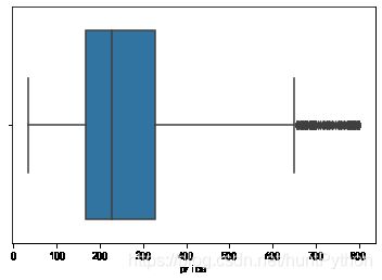
e_data = e_data[e_data['price']>0]#删除价格为0的房源

import seaborn as sns
sns.boxplot(e_data.price,whis=2,orient='h')#选取2倍四分位距仍然有很多异常值，需要删除

def box_plot_outliers(data,data_ser, box_scale):
    iqr = box_scale * (data_ser.quantile(0.75) - data_ser.quantile(0.25))
    val_low = data_ser.quantile(0.25) - iqr
    val_up = data_ser.quantile(0.75) + iqr
    a = data[(data_ser> val_low) & (data_ser<val_up)] #删除异常值
    b = a[['price','neighbourhood']]#由于方差分析只需要各地区因子水平，以及价格，所以删除其他列
    return b
e_data = box_plot_outliers(e_data,e_data.price,2)
e_data

	price	neighbourhood
0	792	朝阳区
2	389	东城区
3	376	东城区
4	537	朝阳区
5	403	东城区
...	...	...
28444	832	延庆县
28446	228	房山区
28447	396	朝阳区
28449	329	朝阳区
28451	295	丰台区

sns.boxplot(e_data.price,whis = 2)

e_data.price.describe()
count    15299.000000
mean       481.556115
std        201.162288
min         54.000000
25%        342.000000
50%        443.000000
75%        584.000000
max       1248.000000
Name: price, dtype: float64

neighbourhood_to_list = {
     '朝阳区':1,
'海淀区':2,
'东城区':3,
'丰台区':4,
'西城区':5,
'通州区':6,
'昌平区':7,
'大兴区':8,
'顺义区':9,
'石景山区':10,
'房山区':11,
'密云县':12,
'门头沟区':13,
'平谷区':14,
'怀柔区':15,
'延庆县':16}

e_data['neighbourhood'] = e_data['neighbourhood'].map(neighbourhood_to_list)
e_data

	price	neighbourhood
0	792	1
2	389	3
3	376	3
4	537	1
5	403	3
...	...	...
28444	832	16
28446	228	11
28447	396	1
28449	329	1
28451	295	4

model = ols('price ~ neighbourhood',e_data).fit()
anovat = anova_lm(model)
print(anovat)
                    df        sum_sq        mean_sq         F    PR(>F)
neighbourhood      1.0  2.967648e+05  296764.791065  7.336672  0.006764
Residual       15297.0  6.187562e+08   40449.511263       NaN       NaN

可以看到对于全租房来说，房价与地区有强烈的显著相关性。

2.Private room 下地区对房租价格的影响

p_data = data[data['room_type'] == 'Private room']
p_data.price.describe()
count     9838.000000
mean       430.681236
std       1203.643527
min          0.000000
25%        181.000000
50%        248.000000
75%        389.000000
max      66667.000000
Name: price, dtype: float64

p_data = p_data[p_data['price']>0]
p_data = box_plot_outliers(p_data,p_data.price,2)
sns.boxplot(p_data.price,whis = 2)

p_data['neighbourhood'] = p_data['neighbourhood'].map(neighbourhood_to_list)
model = ols('price ~ neighbourhood',p_data).fit()
anovat = anova_lm(model)
print(anovat)
                   df        sum_sq       mean_sq           F         PR(>F)
neighbourhood     1.0  1.294708e+07  1.294708e+07  593.986554  4.194081e-127
Residual       9002.0  1.962160e+08  2.179693e+04         NaN            NaN

3. Shared room 下地区对房租价格的影响

s_data = data[data['room_type'] == 'Shared room']
s_data.price.describe()
count     1658.000000
mean       293.343185
std       2521.130124
min         27.000000
25%         87.000000
50%        107.000000
75%        148.000000
max      67909.000000
Name: price, dtype: float64

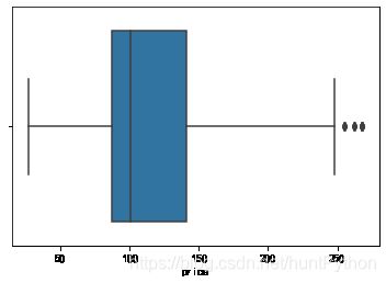
s_data = box_plot_outliers(s_data,s_data.price,2)
sns.boxplot(s_data.price,whis = 2)

p_data['neighbourhood'] = p_data['neighbourhood'].map(neighbourhood_to_list)
model = ols('price ~ neighbourhood',s_data).fit()
anovat = anova_lm(model)
print(anovat)
                   df        sum_sq      mean_sq         F   PR(>F)
neighbourhood    13.0  7.287987e+04  5606.144166  2.838746  0.00048
Residual       1503.0  2.968225e+06  1974.866697       NaN      NaN

单因子方差分析完毕