R语言排序分析(PCA、CA、PCoA、NMDS、RDA)
文章目录
-
- ****排序 Ordination****
- 非约束性排序
-
- PCA
- CA
- PCoA
- NMDS
- **RDA约束性排序**
-
- ggplot可视化
- ggvegan可视化
- rda.plot()函数
排序 Ordination
按照有无解释变量,可分为非约束性排序(unconstrained ordination)与约束性排序(constrained ordination)。
非约束性排序
- PCA 线性模型,基于原始矩阵
- CA 单峰模型,基于原始矩阵
- PCoA 基于原始距离矩阵
- NMDS 基于秩和距离矩阵
- Clustering
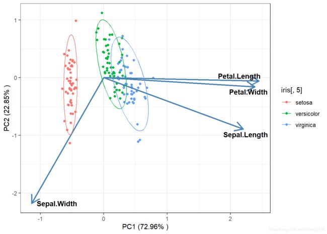
PCA
PCA计算的是欧氏距离。
library(vegan)
library(tidyverse)
library(ggpubr)
#l对iris做PCA
model_pca<-rda(iris[,-5],scale=T,scaling=1)
#提取特征值与方差解释度%
summary(model_pca)$cont$importance #特征值与方差解释度
## Importance of components:
##                          PC1    PC2     PC3      PC4
## Eigenvalue            2.9185 0.9140 0.14676 0.020715
## Proportion Explained  0.7296 0.2285 0.03669 0.005179
## Cumulative Proportion 0.7296 0.9581 0.99482 1.000000
#载荷矩阵loading
head(model_pca$CA$v)
##                     PC1         PC2        PC3        PC4
## Sepal.Length  0.5210659 -0.37741762  0.7195664  0.2612863
## Sepal.Width  -0.2693474 -0.92329566 -0.2443818 -0.1235096
## Petal.Length  0.5804131 -0.02449161 -0.1421264 -0.8014492
## Petal.Width   0.5648565 -0.06694199 -0.6342727  0.5235971
#site scores
sites_score<-scores(model_pca,display = "sites")%>%
  as.data.frame()%>%
  rownames_to_column()%>%
  as_tibble()
sites_score
## # A tibble: 150 x 3
##    rowname    PC1     PC2
##
##  1 sit1    -0.535 -0.203
##  2 sit2    -0.491  0.284
##  3 sit3    -0.558  0.144
##  4 sit4    -0.543  0.252
##  5 sit5    -0.564 -0.273
##  6 sit6    -0.490 -0.628
##  7 sit7    -0.577 -0.0201
##  8 sit8    -0.527 -0.0942
##  9 sit9    -0.551  0.471
## 10 sit10   -0.516  0.198
## # ... with 140 more rows
#specoes scores
species_score<-scores(model_pca,display = "species")%>%
  as.data.frame()%>%
  rownames_to_column()%>%
  as_tibble()
species_score
## # A tibble: 4 x 3
##   rowname        PC1     PC2
##
## 1 Sepal.Length  2.20 -0.891
## 2 Sepal.Width  -1.14 -2.18
## 3 Petal.Length  2.45 -0.0578
## 4 Petal.Width   2.38 -0.158
#可视化
  ggplot()+
    geom_point(data=sites_score,aes(x=PC1,y=PC2,color=iris[,5]))+
    labs(x=paste("PC1 (",round(summary(model_pca)$cont$importance [2,1]*100,2)
                 ,"% )",sep=""),
         y=paste("PC2 (",round(summary(model_pca)$cont$importance [2,2]*100,2)
                 ,"% )",sep=""))+
    geom_segment(data=species_score,aes(x=0,y=0,xend=PC1,yend=PC2),size = 1,
                 arrow = arrow(length = unit(0.2, "inches")),color="steelblue")+
    ggrepel::geom_text_repel(data=species_score,nudge_x = 0.4,
                             fontface="bold", color="black",
                             aes(x=PC1,y=PC2,label=rowname))+
    stat_ellipse(type="norm",level= 0.9,
                  data=sites_score,aes(x=PC1,y=PC2,color=iris[,5]))+
    theme_bw()
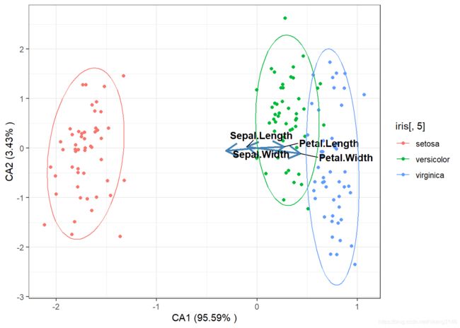
CA
CA计算用的是卡方距离。
#l对iris做PCA
model_ca<-cca(iris[,-5],scale=T,scaling=1)
#提取特征值与方差解释度%
summary(model_ca)$cont$importance #特征值与方差解释度
## Importance of components:
##                           CA1     CA2       CA3
## Eigenvalue            0.06129 0.00220 0.0006302
## Proportion Explained  0.95585 0.03432 0.0098288
## Cumulative Proportion 0.95585 0.99017 1.0000000
#载荷矩阵loading
head(model_ca$CA$v)
##                     CA1        CA2        CA3
## Sepal.Length -0.4118927  0.6554888  0.8787892
## Sepal.Width  -1.2425352 -1.0612937 -0.9286927
## Petal.Length  1.0958023  0.5920802 -1.0659541
## Petal.Width   1.7406720 -2.3434255  1.4258929
#site scores
sites_score<-scores(model_ca,display = "sites")%>%
  as.data.frame()%>%
  rownames_to_column()%>%
  as_tibble()
sites_score
## # A tibble: 150 x 3
##    rowname   CA1     CA2
##
##  1 sit1    -1.81 -0.0236
##  2 sit2    -1.64  0.871
##  3 sit3    -1.78 -0.0325
##  4 sit4    -1.61  0.328
##  5 sit5    -1.84 -0.382
##  6 sit6    -1.60 -0.992
##  7 sit7    -1.69 -1.03
##  8 sit8    -1.72  0.187
##  9 sit9    -1.60  0.399
## 10 sit10   -1.71  1.28
## # ... with 140 more rows
#species scores
species_score<-scores(model_ca,display = "species")%>%
  as.data.frame()%>%
  rownames_to_column()%>%
  as_tibble()
species_score
## # A tibble: 4 x 3
##   rowname         CA1     CA2
##
## 1 Sepal.Length -0.102  0.0307
## 2 Sepal.Width  -0.308 -0.0498
## 3 Petal.Length  0.271  0.0278
## 4 Petal.Width   0.431 -0.110
#plot
ggplot()+
    geom_point(data=sites_score,aes(x=CA1,y=CA2,color=iris[,5]))+
    labs(x=paste("CA1 (",round(summary(model_ca)$cont$importance [2,1]*100,2)
                 ,"% )",sep=""),
         y=paste("CA2 (",round(summary(model_ca)$cont$importance [2,2]*100,2)
                 ,"% )",sep=""))+
    geom_segment(data=species_score,aes(x=0,y=0,xend=CA1,yend=CA2),size = 1,
                 arrow = arrow(length = unit(0.2, "inches")),color="steelblue")+
    ggrepel::geom_text_repel(data=species_score,nudge_x = 0.4,
                             fontface="bold", color="black",
                             aes(x=CA1,y=CA2,label=rowname))+
    stat_ellipse(type="norm",level= 0.9,
                  data=sites_score,aes(x=CA1,y=CA2,color=iris[,5]))+

    theme_bw()
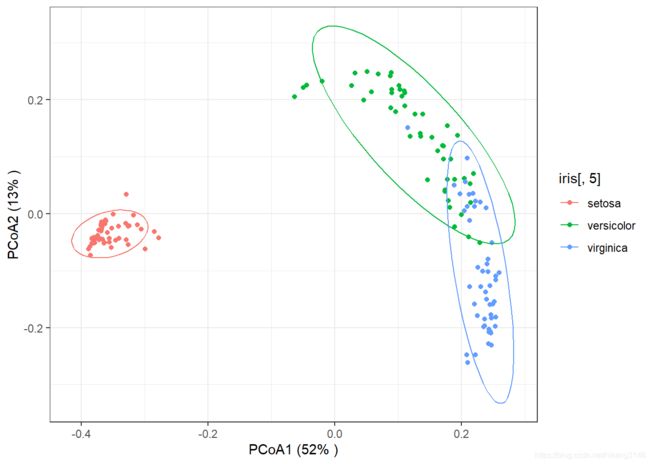
PCoA
PCoA可以采用其它距离矩阵(非欧式、卡方距离),如Bray-Cuurtis距离等。
#为防止出现大量负值特征值,需要对距离开方转换
model_pcoa<-vegdist(iris[,1:4],method="jaccard")%>% #计算距离
  sqrt()%>% #平方根转换
  cmdscale(k=2,eig=T) #多维标度转换

#变异解释
pcoa_explain<-round(model_pcoa$eig/sum(model_pcoa$eig)*100)
pcoa_explain
##   [1] 52 13  5  4  3  2  2  2  1  1  1  1  1  1  1  1  1  1  0  0  0  0  0  0  0  0  0
##  [28]  0  0  0  0  0  0  0  0  0  0  0  0  0  0  0  0  0  0  0  0  0  0  0  0  0  0  0
##  [55]  0  0  0  0  0  0  0  0  0  0  0  0  0  0  0  0  0  0  0  0  0  0  0  0  0  0  0
##  [82]  0  0  0  0  0  0  0  0  0  0  0  0  0  0  0  0  0  0  0  0  0  0  0  0  0  0  0
## [109]  0  0  0  0  0  0  0  0  0  0  0  0  0  0  0  0  0  0  0  0  0  0  0  0  0  0  0
## [136]  0  0  0  0  0  0  0  0  0  0  0  0  0  0  0
#可视化
ggplot()+
  geom_point(aes(x=model_pcoa$points[,1],
                 y=model_pcoa$points[,2],
                 color=iris[,5]))+
  labs(x=paste("PCoA1 (",pcoa_explain[1],"% )",sep=""),
         y=paste("PCoA2 (",pcoa_explain[2],"% )",sep=""))+
  stat_ellipse(type="norm",level= 0.9,
                  aes(x=model_pcoa$points[,1],
                      y=model_pcoa$points[,2],color=iris[,5]))+
  theme_bw()
NMDS
NMDS对距离采用rank排序的方式处理。
According to Clarke and Warwick 2001:
- stress < 0.05: excellent representation
- stress < 0.1: good representation
- stress < 0.2: acceptable representation
- stress > 0.3: unsatisfactory representation
model_nmds<-metaMDS(iris[,-5],distance="bray")
print(model_nmds$stress)
## [1] 0.03775523
# NMDS可视化
ggplot()+
  geom_point(aes(x=model_nmds$points[,1],y=model_nmds$points[,2],color=iris[,5]))+
  labs(x="NMDS1",y="NMDS2")+
  annotate(geom='text',x=median(model_nmds$points[,2]),
           y=max(model_nmds$points[,2]),
           label=paste("stress=",round(model_nmds$stress,3),sep=""))+
  stat_ellipse(type="norm",level= 0.9,
                  aes(x=model_nmds$points[,1],
                      y=model_nmds$points[,2],color=iris[,5]))+
  theme_bw()

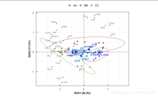
RDA约束性排序
RDA结合了线性回归与PCA主成分分析,是目前生态学常用的探索环境变量与群落组成关系的统计方法,具体分析原理可参考《Numerical Ecology》。对RDA的原理、操作已有很多文章介绍,此处不再赘言,本文着重在可视化部分
library(vegan)
data(dune)
data(dune.env)
model_rda<-rda(dune~.,data=dune.env,scale=T)
explain<-round(summary(eigenvals(model_rda))[2,1:2]*100) #explain%
rda_scores<-scores(model_rda,display=c("wa","sp","bp","cn"),scaling=1)
rda_scores$sites
rda_scores$species
RDA分析结果中最主要的是提取site、species、env的得分,可用scores()函数提取,分析结果也可用summary(rda_model)查看。
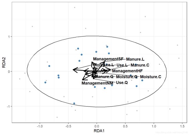
ggplot可视化
rda_scores_biplot<-rda_scores$biplot%>%as.data.frame()%>%rownames_to_column()%>%as_tibble()
ggplot()+
  geom_point(data=as.data.frame(rda_scores$sites),
             aes(x=RDA1,y=RDA2),color="steelblue",size=2)+
  stat_ellipse(data=as.data.frame(rda_scores$sites),
               aes(x=RDA1,y=RDA2),type="norm",level= 0.9)+
  geom_point(data=as.data.frame(rda_scores$species),
             aes(x=RDA1,y=RDA2),color="gray",size=1)+
  geom_segment(data=as.data.frame(rda_scores_biplot),
               aes(x=0,y=0,xend=RDA1,yend=RDA2),
               size = 1,arrow = arrow(length = unit(0.2, "inches")),color="black")+
  ggrepel::geom_text_repel(
    data=rda_scores_biplot,
    aes(x=RDA1,y=RDA2,label=rowname),
    nudge_x = 0.4,fontface="bold", color="black")+
    theme_bw()
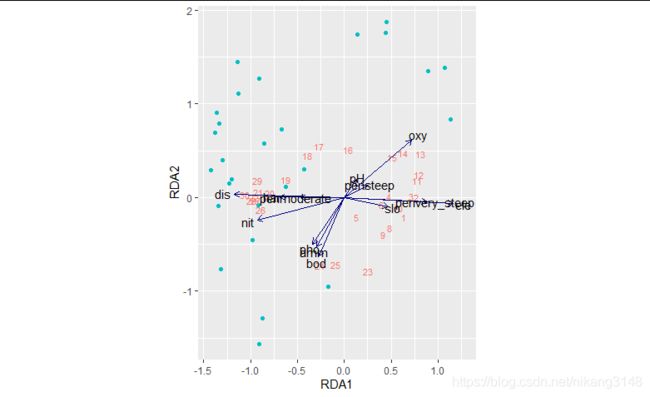
ggvegan可视化
比较方便的有ggvegan包(github安装),看着也还行,但是还是很多参数可调。
autoplot(spe.rda2,legend.position="none",
         layers=c("sites","species","biplot"),
         geom=c("text","point"),arrow=F,
         scaling="sites"
         )
rda.plot()函数
脱离ggvegan包,用ggplot绘图函数打包成函数,并用ggpubr包简化颜色设置。
rda.plot(spe.rda2,
         scaling=1, #scaling code 1-3
         display=c("sp","sites","env","cn"), #choose scores here
         group=spe.tr, #treatments
         palette = "igv", #see ggsci
         envcol=get_palette("jco",8)[1], # envrionemtal variables see ggpubr
         cncol="blue", #factors color
         ellipse = T,
         ellipse.type="norm",
         ellipse.level=0.9
         ) #draw ellipe