【ZJU-Machine Learning】卷积神经网络-LeNet
卷积神经网络的概念
由手工设计卷积核变成了自动学习卷积核。
何为卷积核?
我们在《信号与系统》中学到很多变换,如小波变换,傅里叶变换等。
对于傅里叶变换:

对于傅里叶变换中的卷积核,他的作用是,和f(t)信号进行作用(这个作用就是先乘起来再加起来)
而我们学到这些变换,就是为了人为的找一个卷积核。
而对于图像处理,就是为了将卷积核和图像作用,产生一个特征,我们用多个卷积核提取多个特征。
术语

步长与特征图大小的关系


补零
对于一部分步长(一般是大于1的),可能卷积核无法遍历到其边缘部分,导致其无法参加运算,我们对其边缘部分进行补零,以防浪费像素。

权值共享
可以将图像卷积看成全连接网络的权值共享(weight sharing)
、

上面的卷积操作,等价于如下权值共享网络:


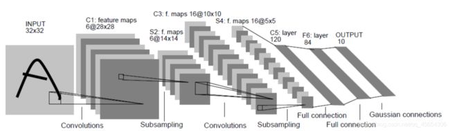
LeNet
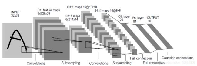
第一步
要注意非线性变换(Relu)

第二步
对2*2的范围进行取平均,然后进行Relu变换。
反向传播时,对参数的偏导取1/4填入前面的神经元就可以。
第三步
用16个5 * 5 * 6的卷积核,Stride=1,作用到14 * 14 * 6的特征图上,得出16个10 * 10的特征图
第四步
取平均
第五步
将上面的16 * 5 * 5输入全连接层。

可以看出,整个网络的训练速度取决于卷积层(时间复杂度),参数个数取决于全连接层(空间复杂度)。
注意:所有线性变换后,要接着一个ReLu
Tensorflow实现LENET-5
第1层(CONV1)和第2层(AVG_POOL1)
sess = tf.InteractiveSession()
x = tf.placeholder(“float”, shape=[None, 784])
y_ = tf.placeholder(“float”, shape=[None, 10])

W_conv1 = weight_variable([5, 5, 1, 6])
b_conv1 = bias_variable([6])

x_image = tf.reshape(x, [-1,28,28,1])
h_conv1 = tf.nn.relu(conv2d(x_image, W_conv1,’SAME’) + b_conv1)
h_pool1 = average_pool_2x2(h_conv1)
def conv2d(x, W, padding_method='SAME'):
	 return tf.nn.conv2d(x, W, strides=[1, 1, 1, 1], padding=padding_method)
def avg_pool_2x2(x, padding_method='SAME'):
  return tf.nn.avg_pool(x, ksize=[1, 2, 2, 1],
     strides=[1, 2, 2, 1], padding= padding_method)
第3层(CONV2)和第4层(AVG_POOL2)
W_conv2 = weight_variable([5, 5, 6, 16])
b_conv2 = bias_variable([16])

h_conv2 = tf.nn.relu(conv2d(h_pool1, W_conv2) + b_conv2)
h_pool2 = avg_pool_2x2(h_conv2)
三个全连接层
W_fc1 = weight_variable([5 * 5 * 16, 120])
b_fc1 = bias_variable([120])

h_pool2_flat = tf.reshape(h_pool2, [-1, 5*5*16])
h_fc1 = tf.nn.relu(tf.matmul(h_pool2_flat, W_fc1) + b_fc1)

keep_prob = tf.placeholder("float")
h_fc1_drop = tf.nn.dropout(h_fc1, keep_prob)
W_fc2 = weight_variable([120, 84])
b_fc2 = bias_variable([84])
h_fc2 =tf.nn.relu(tf.matmul(h_fc1_drop, W_fc2) + b_fc2)
h_fc2_drop = tf.nn.dropout(h_fc2, keep_prob)

W_fc3 = weight_variable([84, 10])
b_fc3 = bias_variable([10])

y_conv=tf.nn.softmax(tf.matmul(h_fc2_drop, W_fc3) + b_fc3)
cross_entropy = -tf.reduce_sum(y_*tf.log(y_conv))
train_step = tf.train.AdamOptimizer(1e-4).minimize(cross_entropy)correct_prediction = tf.equal(tf.argmax(y_conv,1), tf.argmax(y_,1))
accuracy = tf.reduce_mean(tf.cast(correct_prediction, "float"))

sess.run(tf.global_variables_initializer())

for i in range(10000):
	batch = mnist.train.next_batch(50)
	if i%100 == 0:
	    train_accuracy = accuracy.eval(feed_dict={
     x:batch[0], y_: batch[1], keep_prob: 1.0})
	    print "step %d, training accuracy %g"%(i, train_accuracy)
	    train_step.run(feed_dict={
     x: batch[0], y_: batch[1], keep_prob: 0.5})
	    print "test accuracy %g"%accuracy.eval(feed_dict={

	    x: mnist.test.images, y_: mnist.test.labels, keep_prob: 1.0})
Caffe实现LENET-5
使用Caffe训练神经网络有三种方式:
- 命令行接口
- Python接口
- Matlab接口
- 命令行接口
Caffe的tools文件夹下有一个Caffe.cpp,写好了训练时参数更新、保存模型等必要的过程。编译好caffe之后,我们在训练的时候只要调用这个可执行文件,并且指定训练的solver即可。
文件结构
1)create_lmdb.sh
2)compute_mean.sh
3)train_lenet.sh
4)lenet_solver.prototxt
5)lenet_train_test.prototxt
6)test_lenet.sh
主要代码实现
- create_lmdb.sh
DATA=/home/hty/caffe-master/examples/mnist
BUILD=/home/hty/caffe-master/build/tools

rm -rf $DATA/mnist_train_lmdb
rm -rf $DATA/mnist_test_lmdb

$BUILD/convert_imageset --shuffle \
--resize_height=28 --resize_width=28 \
$DATA/    \
$DATA/training.txt  $DATA/mnist_train_lmdb

$BUILD/convert_imageset --shuffle \
--resize_height=28 --resize_width=28 \
$DATA/    \
$DATA/testing.txt  $DATA/mnist_test_lmdb
- compute_mean.sh
#!/usr/bin/env sh
# This script converts the mnist data into lmdb/leveldb format,
# depending on the value assigned to $BACKEND.
set -e

DATA=/home/hty/caffe-master/examples/mnist
BUILD=/home/hty/caffe-master/build/tools

rm -rf $DATA/mean.binaryproto

$BUILD/compute_image_mean $DATA/mnist_train_lmdb $DATA/mean.binaryproto $@
- train_lenet.sh
#!/usr/bin/env sh
set -e

BUILD=/home/hty/caffe-master/build/tools
DATA=/home/hty/caffe-master/examples/mnist
$BUILD/caffe train --solver=$DATA/lenet_solver.prototxt $@
- lenet_solver.prototxt
net: "examples/mnist/lenet_train_test.prototxt"
# test_iter specifies how many forward passes the test should carry out.
# In the case of MNIST, we have test batch size 100 and 100 test iterations,
# covering the full 10,000 testing images.
test_iter: 100
# Carry out testing every 500 training iterations.
test_interval: 500
# The base learning rate, momentum and the weight decay of the network.
base_lr: 0.01
momentum: 0.0
weight_decay: 0.0005
# The learning rate policy
lr_policy: "inv"
gamma: 0.0001
power: 0.75
# Display every 100 iterations
display: 100
# The maximum number of iterations
max_iter: 10000
# snapshot intermediate results
snapshot: 5000
snapshot_prefix: "examples/mnist/lenet_rmsprop"
# solver mode: CPU or GPU
solver_mode: GPU
type: "RMSProp"
rms_decay: 0.98
Lr_policy介绍
fixed: always return base_lr.
step: return base_lr * gamma ^ (floor(iter / step))
exp: return base_lr * gamma ^ iter
inv: return base_lr * (1 + gamma * iter) ^ (- power)
multistep: similar to step but it allows non uniform steps defined by  stepvalue
poly: the effective learning rate follows a polynomial decay, to be  zero by the max_iter. return base_lr (1 - iter/max_iter) ^ (power)
sigmoid: the effective learning rate follows a sigmod decay  return base_lr ( 1/(1 + exp(-gamma * (iter - stepsize))))
where base_lr, max_iter, gamma, step, stepvalue and power are defined  in the solver parameter protocol buffer, and iter is the current iteration.
- lenet_train_test.prototxt
layer {

  name: "conv1"
  type: "Convolution"
  bottom: "data"
  top: "conv1“
 param {

    lr_mult: 1
  }
  param {

    lr_mult: 2
  }
  convolution_param {

    num_output: 6
    kernel_size: 5
    stride: 1
    weight_filler {

      type: "xavier"
    }
    bias_filler {

      type: "constant"
    }
  }
}
layer {

 name: "pool1“
   type: "Pooling“
   bottom: "conv1“
   top: "pool1“
   pooling_param {

   pool: MAX
   kernel_size: 2
   stride: 2
 }
}
layer {

  name: "loss"
  type: "SoftmaxWithLoss"
  bottom: "ip2"
  bottom: "label"
  top: "loss"
  include {

    phase: TRAIN
  }
}
6.test_lenet.sh
#!/usr/bin/env sh
set -e

BUILD=/home/hty/caffe-master/build/tools
DATA=/home/hty/caffe-master/examples/mnist
$BUILD/caffe test -model $DATA/lenet_train_test.prototxt -weights $DATA/lenet_iter_10000.caffemodel -iterations 100 $@
Caffe的优缺点
Caffe的优点
- 非常适合卷积神经网络做图像识别
- 预训练的model比较多
- 代码量少
- 封装比较少,源程序容易看懂,容易修改
- 训练好的参数容易导出到其他程序文件 (如C语言)
- 适合工业应用
Caffe的缺点
- 由于是专门为卷积神经网络开发的,结构不灵活,难以进行其他应用。
- 代码写法比较僵化,每一层都要写。
- 除非修改源码,否则不能完全调节所有细节。