机器学习--决策树
文章目录
-
- 决策树的思想
- 分类树
-
- 信息熵
-
- 信息增熵
- 基尼系数
- CART
- 简单实现
-
- CART剪枝
- sklearn的分类树
- 回归树
-
- CART
- sklearn的回归树
决策树的思想
决策树的思想在现实中也非常常见,比如买一个东西,我们在想买或者不买,就会经过类似以下的决策过程: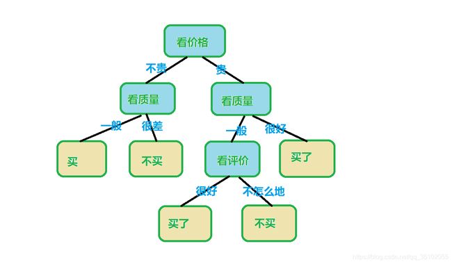
决策树也是如此,比如我们要解决一个分类问题,也可以借助类似的过程,然后对输入的数据进行分类。
在分类树中每一个叶节点都是一个类别,而每一个内部节点对应着一个规则条件。
分类树
分类树就是用来解决分类问题的决策树。
一颗决策树的学习过程分为:特征选择,决策树的生成,剪枝
三个过程
信息熵
首先是特征选择,每次决策树进行分支其实都是选择一个特征然后根据这个特征进行分支。
而我们选择特征时,有的特征可能用于当前的节点划分十分有效,有的则几乎无法用于当前节点的划分,所以需要一个标准进行衡量某个特征进行划分之后它的划分效果好坏如何。
首先介绍信息熵,信息熵可以衡量随机变量的不确定度。
设X是一个取有限个值的离散随机变量且有:
P ( X = x i ) = p i ( i = 1 , 2... , n ) P(X=x_i)=p_i(i=1,2...,n) P(X=xi)=pi(i=1,2...,n)
则这个随机变量X的信息熵就为:
H ( x ) = − ∑ i = 1 n p i l o g ( p i ) H(x) = -\sum\limits_{i = 1}^np_ilog(p_i) H(x)=−i=1∑npilog(pi)
其中,这个对数如果以2为底则信息熵此时的单位为比特,以e为底则此时单位为纳特,并且如果存在 p i = 0 p_i=0 pi=0则默认 p i l o g ( p i ) = 0 p_ilog(p_i)=0 pilog(pi)=0
举个例子,假设有一个只有两个类别的样本,一个类别为1一个为0,其中1这个类别占 1 3 \frac{1}{3} 31,0这个类别占 2 3 \frac{2}{3} 32则信息熵则为
H ( x ) = − [ 1 3 l o g 2 ( 1 3 ) + 2 3 l o g 2 ( 2 3 ) ] ≈ 0.918 H(x) = -[\frac{1}{3}log_2(\frac{1}{3}) + \frac{2}{3}log_2(\frac{2}{3})] \approx 0.918 H(x)=−[31log2(31)+32log2(32)]≈0.918
信息熵越大说明分类越不准确,也就是此时混乱程度越大,小则相反。
假设随机变量X只有两个类别(即只有两种取值),则设取其中一个类别的概率为 a a a则另一个就为 1 − a 1-a 1−a
此时信息熵就为
H ( x ) = − [ a ∗ l o g 2 ( a ) + ( 1 − a ) ∗ l o g 2 ( 1 − a ) ] H(x) = -[a*log_2(a)+ (1 - a) * log_2(1-a)] H(x)=−[a∗log2(a)+(1−a)∗log2(1−a)]
此时可以画出它的图像。

可以发现当a的取等于1或者0时信息熵的值都取到了最小,切当a取到了0.5时信息熵最大。
也很容易理解,因为当a=0.5时X的取值最不确定,而等于0或者1时,X的取值最确定。
信息增熵
首先定义条件熵,条件熵 H ( Y ∣ X ) H(Y|X) H(Y∣X)是指在随机变量X已经确定了的条件下,Y的不确定性,其定义为:
H ( Y ∣ X ) = ∑ i = 1 n p i H ( Y ∣ X = i ) H(Y|X)=\sum\limits_{i = 1}^np_iH(Y|X=i) H(Y∣X)=i=1∑npiH(Y∣X=i)
其中 p i = P ( X = i ) p_i=P(X=i) pi=P(X=i)
此时就可以定义信息增熵了:
设训练集为 D D D,当前所选的特征为A,则选特征A之后的信息增熵为
G ( D , A ) = H ( D ) − H ( D ∣ A ) G(D, A)=H(D) - H(D|A) G(D,A)=H(D)−H(D∣A)
即在选择特征A之后并且划分,然后得到的训练集的信息熵与原本训练集的信息熵的差,这个差越大训练集的信息熵减少的就越多,划分出来的数据的种类就越确定,划分效果就越好。
基尼系数
基尼系数与信息熵类似,也可以用于计算当前训练集的不确定度,它的计算公式为
G i n i ( p ) = 1 − ∑ i = 1 n p i 2 Gini(p)=1-\sum\limits_{i = 1}^np_i^2 Gini(p)=1−i=1∑npi2
CART
CART的全称为Classification and Regression Tree.
CART是实现决策树的算法之一,他假设决策树每个内部节点只有"是"或者"否"两种状态,这样所得到的决策树就是一颗二叉树。
CART算法包括两部分
- 基于训练数据生成决策树,生成的决策树要尽可能的大。
- 用验证数据集对决策树进行剪枝,然后选择出最优决策树。
CART树的生成
- 如果当前节点满足条件,则把它作为一个叶节点然后根据少数服从多数确定他的类别。
- 否则,对于每个特征A,选择A所可以取到的所有分隔点 i i i使 A = i A=i A=i然后把训练集D划分成两部分,然后计算信息熵,并选出一个最优的划分。
- 从所有特征中选出信息熵最小的一个划分,然后按这个划分对训练集进行分割
- 对新的划分重复上述步骤,直到满足条件
条件可以有很多,比如当前节点的信息熵小于某个阈值,或者当前节点的样本数小于某个值。
简单实现
首先导入所需要的包
import numpy as np
from collections import Counter
from math import log2
然后定义一个DecisionTree类,重写__inint__方法
class DecisionTree:
    __used_criterion = None
    root = None
    """
    max_depth: 表示最大深度
    criterion: 衡量切分效果的指标[只有'gini'和'entropy']
    min_samples:一个节点被切分所需要的最少样本数
    root用来存树根
    __used_criterion用来存所使用的criterion
    """
    def __init__(self, max_depth=None, criterion='gini', min_samples=10):
        self.max_depth = max_depth
        self.criterion = criterion
        self.min_samples = min_samples
        if criterion == 'gini':
            self.__used_criterion = self.__gini
        else:
            self.__used_criterion = self.__entropy
写出基尼系数和信息熵得到计算公式
def __gini(self, y):
        cout, l = Counter(y), len(y)
        res = 0
        for i in cout.values():
            res += (i / l) ** 2
        return 1 - res

    def __entropy(self, y):
        cout, l = Counter(y), len(y)
        res = 0
        for i in cout.values():
            res += (i / l) * log2(len(i) / l)
然后写一个函数用于切分节点
def __splitFeature(self, X, y, id): # id表示特征,X和y是data和target
        lX, rX, ly, ry = None, None, None, None # 表示切分后左右的训练数据,特征
        bestValue, splitLine = float('inf'), None # 最好的值和最好的切分点
        idx = np.argsort(X[:, id]) # 对某个特征所有的值进行排序
        for i in range(1, len(X)):# 这里选取的是依次取每两个点的中间值进行切分,然后选择最好的一个
            tmpSplitLine = (X[idx[i], id] + X[idx[i - 1], id]) / 2
            reIdx = X[:, id] < tmpSplitLine
            reIdxr = X[:, id] >= tmpSplitLine
            tmpValue = self.__used_criterion(y[reIdx]) + self.__used_criterion(y[reIdxr])
            if tmpValue < bestValue:
                splitLine = tmpSplitLine
                bestValue = tmpValue
                lX, rX, ly, ry = X[reIdx], X[reIdxr], y[reIdx], y[reIdxr]
        return lX, rX, ly, ry, bestValue, splitLine
然后我们写一个类用于存储树节点
class TreeNode:
    def __init__(self, split_line=None, c=None):
        self.c = c
        self.feature_position = None
        self.split_line = split_line
        self.left = None
        self.right = None
然后开始递归构建树
def __CART(self, X, y, now: TreeNode, depth):
        # now 是当前正在创建的节点
        L = len(X)
        if L <= self.min_samples or depth == self.max_depth or len(set(y)) == 1: # 如果满足条件就停止然后按照少数服从多数把该节点变成叶节点
            c = Counter(y).most_common()[0][0]
            now.c = c
        else: # 否则进行分割
            minValue = float('inf')
            bestCb, pos = None, None
            for i in range(X.shape[1]):
                cb = self.__splitFeature(X, y, i)
                if cb[4] < minValue:
                    bestCb = cb
                    minValue = cb[4]
                    pos = i
            if not len(cb[0]) or not len(cb[1]): #  处理出现重合点的情况
                c = Counter(y).most_common()[0][0]
                now.c = c
                return
            now.split_line = bestCb[5]
            now.feature_position = pos
            l, r = TreeNode(), TreeNode() # 左右子树的创建
            now.left, now.right = l, r
            self.__CART(bestCb[0], bestCb[2], l, depth + 1)# 递归处理
            self.__CART(bestCb[1], bestCb[3], r, depth + 1)
然后顺便把fit也写出来
def fit(self, X, y):
        self.root = TreeNode() # 创建根节点
        self.__CART(X, y, self.root, 1) # 从根开始递归创建
        return self # 根据sklearn标准返回自身
写一个预测方法
def __single_predict(self, x, now: TreeNode):
        if now.split_line == None: # 如果当前节点没有分隔点那么它是叶节点该输入数据就等于这个类别
            return now.c
        elif x[now.feature_position] < now.split_line: # 否则比较叶节点的指定特征值在切分点的左还是右
            return self.__single_predict(x, now.left)
        else:
            return self.__single_predict(x, now.right)

    def predict(self, X):
        return np.array([self.__single_predict(i, self.root) for i in X])
完整代码
import numpy as np
from collections import Counter
from math import log2

class TreeNode:
    def __init__(self, split_line=None, c=None):
        self.c = c
        self.feature_position = None
        self.split_line = split_line
        self.left = None
        self.right = None


class DecisionTree:
    __used_criterion = None
    root = None

    def __init__(self, max_depth=None, criterion='gini', min_samples=10):
        self.max_depth = max_depth
        self.criterion = criterion
        self.min_samples = min_samples
        if criterion == 'gini':
            self.__used_criterion = self.__gini
        else:
            self.__used_criterion = self.__entropy

    def __gini(self, y):
        cout, l = Counter(y), len(y)
        res = 0
        for i in cout.values():
            res += (i / l) ** 2
        return 1 - res

    def __entropy(self, y):
        cout, l = Counter(y), len(y)
        res = 0
        for i in cout.values():
            res += (i / l) * log2(len(i) / l)
        return -res


    def __splitFeature(self, X, y, id):
        lX, rX, ly, ry = None, None, None, None
        bestValue, splitLine = float('inf'), None
        idx = np.argsort(X[:, id])
        for i in range(1, len(X)):
            tmpSplitLine = (X[idx[i], id] + X[idx[i - 1], id]) / 2
            reIdx = X[:, id] < tmpSplitLine
            reIdxr = X[:, id] >= tmpSplitLine
            tmpValue = self.__used_criterion(y[reIdx]) + self.__used_criterion(y[reIdxr])
            if tmpValue < bestValue:
                splitLine = tmpSplitLine
                bestValue = tmpValue
                lX, rX, ly, ry = X[reIdx], X[reIdxr], y[reIdx], y[reIdxr]
        return lX, rX, ly, ry, bestValue, splitLine

    def __CART(self, X, y, now: TreeNode, depth):
        # now 是当前正在创建的节点
        L = len(X)
        if L <= self.min_samples or depth == self.max_depth or len(set(y)) == 1:
            c = Counter(y).most_common()[0][0]
            now.c = c
        else:
            minValue = float('inf')
            bestCb, pos = None, None
            for i in range(X.shape[1]):
                cb = self.__splitFeature(X, y, i)
                if cb[4] < minValue:
                    bestCb = cb
                    minValue = cb[4]
                    pos = i
            if not len(cb[0]) or not len(cb[1]):
                c = Counter(y).most_common()[0][0]
                now.c = c
                return
            now.split_line = bestCb[5]
            now.feature_position = pos
            l, r = TreeNode(), TreeNode()
            now.left, now.right = l, r
            self.__CART(bestCb[0], bestCb[2], l, depth + 1)
            self.__CART(bestCb[1], bestCb[3], r, depth + 1)

    def fit(self, X, y):
        self.root = TreeNode()
        self.__CART(X, y, self.root, 1)
        return self

    def __single_predict(self, x, now: TreeNode):
        if now.split_line == None:
            return now.c
        elif x[now.feature_position] < now.split_line:
            return self.__single_predict(x, now.left)
        else:
            return self.__single_predict(x, now.right)

    def predict(self, X):
        return np.array([self.__single_predict(i, self.root) for i in X])
CART剪枝
CART剪枝分为两步:
- 对生成的决策树从底端开始不断地向上剪枝,直到根节点,过程中生成一系列子树 { T 0 , T 1 , . . . . , T k } \{T_0, T_1,....,T_k\} { T0,T1,....,Tk}
- 使用交叉验证法在验证集上从子树的集合中选出一个最优子树
设损失函数为
C α ( T ) = C ( T ) + α ∣ T ∣ C_\alpha(T)=C(T) + \alpha|T| Cα(T)=C(T)+α∣T∣
C α ( T ) C_\alpha(T) Cα(T)表示以T为根节点的子树的误差, C ( T ) C(T) C(T)表示以T为根节点的子树其对训练数的误差, α \alpha α是权重, ∣ T ∣ |T| ∣T∣则是以T为根节点的子树的叶子数目。
我们想要剪枝,其目的就是减少叶子的数目从而降低模型的复杂度,所以考虑误差时把叶子的数目也当成一个参数来考量是很合理的。
假设有一个内部点T,设它变成一个叶节点时误差为:
C α ( T ) = C ( T ) + α C_\alpha(T)=C(T) + \alpha Cα(T)=C(T)+α
以他为根的子树 T t T_t Tt的误差为
C α ( T t ) = C ( T t ) + α ∣ T t ∣ C_\alpha(T_t)=C(T_t) +\alpha|T_t| Cα(Tt)=C(Tt)+α∣Tt∣
很明显,当 α \alpha α很小时 C α ( T t ) < C α ( T ) C_\alpha(T_t) < C_\alpha(T) Cα(Tt)<Cα(T),因为构成决策树时分枝之后信息熵或者基尼系数必定减小。
当 α \alpha α 逐渐增大达到某一个值,就会出现 C α ( T t ) = C α ( T ) C_\alpha(T_t) = C_\alpha(T) Cα(Tt)=Cα(T)
此时联立两个式子就有 α = C ( T ) − C ( T t ) ∣ T t ∣ − 1 \alpha=\frac{C(T) - C(T_t)}{|T_t| - 1} α=∣Tt∣−1C(T)−C(Tt)
如果 α \alpha α越小说明这个节点构成的子树删去对整个决策树在训练数据上的偏差增大就越小。
有了上面的几个式子,就可以得到CART剪枝的步骤了。
- 自下而上的计算内部节点 T T T的 C α ( T ) C_\alpha(T) Cα(T)和 C α ( T t ) , ∣ T t ∣ C_\alpha(T_t), |T_t| Cα(Tt),∣Tt∣以及 t m p T = C ( T ) − C ( T t ) ∣ T t ∣ − 1 tmp_T=\frac{C(T) - C(T_t)}{|T_t| - 1} tmpT=∣Tt∣−1C(T)−C(Tt) α = m i n ( α , t m p T ) \alpha=min(\alpha, tmp_T) α=min(α,tmpT)
- 对 t m p T = α tmp_T = \alpha tmpT=α的节点进行剪枝,然后得到剩下的树 T T T并存储
- 如果此时T是由根节点和两个叶节点构成的树那么此时就结束,否则重复上述步骤。
sklearn的分类树
可以从sklearn的tree模块中引入DecisionTreeClassifier
from sklearn.tree import DecisionTreeClassifier
"""
Parameters
    ----------
    criterion :
    	选择使用哪种方式衡量切分效果,可以写'entropy'或者'gini'分别是信息熵和基尼系数
    	实际中使用两个中的哪个都差别不大,但基尼系数计算的比较快一点

    splitter : string, optional (default="best")
        控制如何去选择切分点,可以选'best'和'random',使用best的话会一直生成一种决策树
        使用random则会增加随机性可以防止过拟合,同时也会产生一定的偏差

    max_depth : int or None, optional (default=None)
        决策树的最大深度,用于剪枝

    min_samples_split : int, float, optional (default=2)
        一个样本点被且分时所需要的最小样本数,同样可以用于剪枝,当为浮点数时应该在0-1之间,表示占训练数据
        的比例

    min_samples_leaf : int, float, optional (default=1)
        表示一个叶节点比如包含的最少样本数,当值为浮点数时与min_samples_split同理,也可以用于剪枝

    max_features : int, float, string or None, optional (default=None)
    	用于限制分枝时考虑的特征数,比较暴力的直接舍去特征
        The number of features to consider when looking for the best split:

            - If int, then consider `max_features` features at each split.
            - If float, then `max_features` is a percentage and
              `int(max_features * n_features)` features are considered at each
              split.
            - If "auto", then `max_features=sqrt(n_features)`.
            - If "sqrt", then `max_features=sqrt(n_features)`.
            - If "log2", then `max_features=log2(n_features)`.
            - If None, then `max_features=n_features`.

    random_state : int, RandomState instance or None, optional (default=None)
        用于控制是否随机生成一棵树,如果是则default=None否则可以直接传入一个seed

"""
回归树
CART
CART算法同样可以解决回归问题。
假设CART最终生成n个叶节点 { R 1 , R 2 , . . . , R n } \{R_1, R_2, ..., R_n\} { R1,R2,...,Rn},每个节点有一个预测值 c c c,则有
f ( x i ) = c k ( x i ∈ R k ) f(x_i) = c_k(x_i \in R_k) f(xi)=ck(xi∈Rk)
与分类树一样,我们需要决定如何去切割,需要知道如何计算误差。
回归问题的误差衡量标准很多,这里采用MSE,与分类树一样对于一个内部节点,我们需要选择一个特征,然后找到它的一个最优的切分值,按照这个切分值把训练数据切分成两部分。
假设按照第k个特征以特征值b切分成了两个部分,分别用集合表示为 R 1 ( k , b ) = { x ∣ x k < b } , R 2 ( k , b ) = { x ∣ x k ≥ b } R_1(k, b) =\{x|x_k < b\}, R_2(k, b) =\{x|x_k \geq b\} R1(k,b)={ x∣xk<b},R2(k,b)={ x∣xk≥b}
由于最后每一个叶节点都要有一个预测值,所以对于任意样本数据对应的标记 y 1 , y 2 , . . . , y a y_1, y_2, ...,y_a y1,y2,...,ya想要找到一值w使
∑ i = 1 a ( y i − w ) 2 \sum\limits_{i = 1}^a(y_i - w)^2 i=1∑a(yi−w)2
最小,这个值显然就是 w = 1 a ∑ i = 1 a y i w = \frac{1}{a}\sum\limits_{i = 1}^ay_i w=a1i=1∑ayi。
所以对于某个节点,他的最佳预测值就是这个节点所包含的样本的标记的均值
假设切分后两边数据标记的均值分别为 c 1 , c 2 c_1, c_2 c1,c2,那么求上述最佳切分值就可以表示为求
b ^ = arg min b [ ∑ x i ∈ R 1 ( k , b ) ( y i − c 1 ) 2 + ∑ x i ∈ R 2 ( k , b ) ( y i − c 2 ) 2 ] \hat b=\argmin_{b}[\sum\limits_{x_i \in R_1(k, b)}(y_i - c_1)^2 + \sum\limits_{x_i \in R_2(k, b)}(y_i - c_2)^2] b^=bargmin[xi∈R1(k,b)∑(yi−c1)2+xi∈R2(k,b)∑(yi−c2)2]
然后再求出最佳的一个用于切分的特征
k ^ , b ^ = arg min k , b [ ∑ x i ∈ R 1 ( k , b ) ( y i − c 1 ) 2 + ∑ x i ∈ R 2 ( k , b ) ( y i − c 2 ) 2 ] \hat k, \hat b = \argmin_{k, b}[\sum\limits_{x_i \in R_1(k, b)}(y_i - c_1)^2 + \sum\limits_{x_i \in R_2(k, b)}(y_i - c_2)^2] k^,b^=k,bargmin[xi∈R1(k,b)∑(yi−c1)2+xi∈R2(k,b)∑(yi−c2)2]
然后把切分后的数据传入两个孩子中,然后递归重复上述步骤。
sklearn的回归树
sklearn中从tree模块导入DecisionTreeRegressor,就可以使用回归树了。
回归树的参数和分类树很相似,就不写了,生成一个伪数据测试一下回归树的拟合效果。
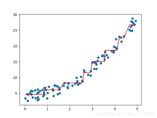
可以发现决策树的对于这么一个数据它的偏差很大,但是后续可以通过集成学习的方法来增强它的拟合能力比如随机森林,GBDT