数独项目第二弹:图像处理pian
数独项目第二弹:图像处理pian
- 前言
- 必备库+导入图片
- 轮廓检测+角点获取
- 仿射变换
- 直线检测
- DFS连通域检测+操刀裁剪
- 总结
- Reference
前言
哈喽,小刀又来咕咕咕了,上次我们讲到利用 DFS来解决九宫格填数的问题,还说要做一个比较完整的小项目,好滴,这个坑挖好了,今天继续填!
友情提醒:今天的推文不短且有点硬核风,希望想认真看的小朋友找个空闲的时间认真阅读~

这次我们来讲解怎么用比较通用性的图像处理方法把一张九宫格题目的图片裁剪出我们想要的含有数字的区域
必备库+导入图片
这次我们需要用到的出装有:
import os
import cv2 as cv
import numpy as np
import matplotlib.pyplot as plt
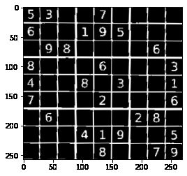
假设我们有下面的一张图:
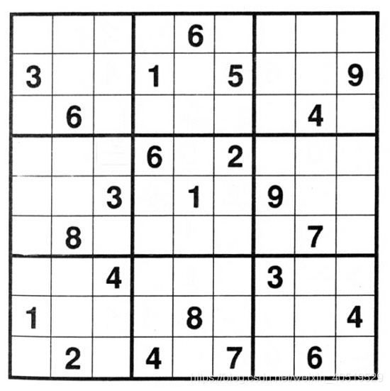
记住我们的目的是为了裁剪出我们需要的数字,这样方方正正的图自然很好处理,等下我也会展示怎么处理有畸变的图像
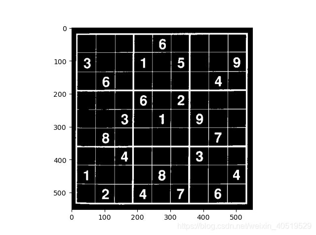
首先我们读取该图像,然后进行取反(一般希望目标是白色,背景是黑色,方便后续操作)和二值操作(像canny或者findContours这些函数都是需要二值滴)
# 读取图像
img = cv.imread(img_name)
# cvtColor进行色彩空间转换:彩色图到灰色图
gray_img = cv.cvtColor(img, cv.COLOR_BGR2GRAY)
# 取反灰度值
gray_img = ~gray_img
# 二值化阈值
threshold = 127  # np.mean(gray_img)
# 二值化
ret, thresh_img = cv.threshold(gray_img, 127, 255, cv.THRESH_BINARY)
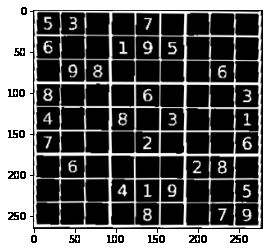
结果如下:
根据九宫格的特点就是行列组成规整的矩形,所以我们只要找到九宫格所在的矩形框,并且平铺没有明显畸变,就可以来分割啦(案板上的九宫格,任你宰割
那就又回到CV里经典到不能再经典的轮廓查找,矩形框角点获取和直线检测等问题啦
轮廓检测+角点获取
# 轮廓查找函数(具体函数用法大家可以官网查询:)
contours,hierarchy = cv.findContours(erode_img, cv.RETR_TREE, cv.CHAIN_APPROX_NONE)
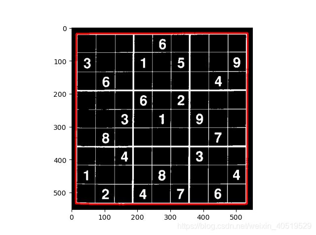
# 一般是最长的轮廓,即九宫格最外边的大矩形
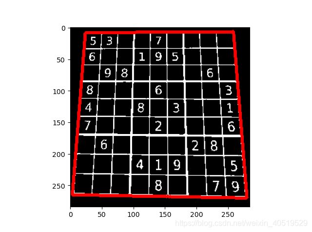
# 画一下矩形框看看对不对
img_copy = cv.cvtColor(np.copy(thresh_img),cv.COLOR_GRAY2BGR)
img_copy_contour = cv.drawContours(img_copy,contours,np.argmax(contours_len),(0,0,255,),3)
结果如下:
获取四个顶点也是有函数滴,可以用角点检测,但是对这种方方正正的,我们直接用最小外包矩形也可以得到比较好的效果:
min_rect = cv.minAreaRect(contours[np.argmax(contours_len)])
rect_points = cv.boxPoints(min_rect).tolist()
sum_p = [sum(p) for p in rect_points]
# tl:top_left tr:top_right
# br:bottom_right bl:bottom_left
# 左上顶点坐标和最小,右下顶点坐标和最大
tl = rect_points[sum_p.index(min(sum_p))]
br = rect_points[sum_p.index(max(sum_p))]
# 剩下的顶点为左下和右上,根据x的大小区分
temp = sorted([r for r in rect_points if r != tl and r != br], key=lambda x: x[0])
bl = temp[0]
tr = temp[1]
# re_group
rect_points = [tl, tr, br, bl]
print(rect_points)

"""
[output]
[[12.0, 16.0], [534.0, 16.0], [534.0, 536.0], [12.0, 536.0]]
"""
我们来看看找得对不对:
for r in rect_points:
    cv.circle(img_copy, tuple(r), 5, (0,0,255), 3)

plt.figure(1)
plt.title('check corner coordinates')
plt.imshow(cv.cvtColor(img_copy, cv.COLOR_BGR2RGB))
plt.show()

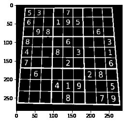
接下来我们来看看有线性畸变的图像怎么处理,比如下面这张图:
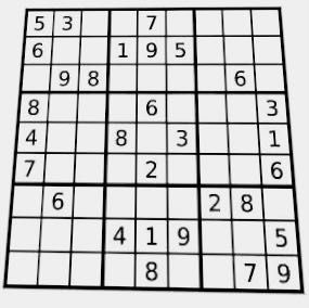
可以看到有明显的纵向拉伸,这个时候我们不能再用上面cv.minAreaRect函数来进行查找最小外包矩形,因为这样得不到真实的九宫格外部矩形角点,后续的仿射变换也会错误,当然啦,这种情况也有方法:
首先我们通过轮廓查找找到ROI(兴趣即目标)区域:
轮廓查找莫得问题,接着我们来进行角点的提取,这里用到的是多边形逼近拟合函数cv.approxPolyDP
"""
approxCurve	=	cv.approxPolyDP(curve, epsilon, closed[, approxCurve])
curve: 2D点集,即待拟合的轮廓点
approxCurve: 多边形拟合的结果
epsilon: 精度,表示拟合结果与原轮廓的最大容许距离
closed: 轮廓是否是闭合的
"""
rect_points = cv.approxPolyDP(contours[np.argmax(contours_len)], 0.02 * cv.arcLength(contours[np.argmax(contours_len)], closed=True), closed=True)
print(rect_points)

"""
[output]
[[[258   6]]
 [[23   9]]
 [[3 265]]
 [[280 269]]]
 """
这里我们的轮廓本来就是拉扯后的矩形,所以结果应该是四个角点,容许精度我们设置为原轮廓周长的0.02(cv.arcLength可以求取一段轮廓的周长
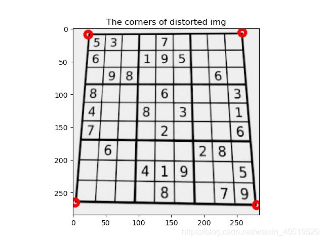
注意这里的points的大小是 (4, 1, 2),我们来显示在原图上一波:
img_copy=np.copy(img)
for r in rect_points:
    # 半径为5个像素,颜色为红色,线宽为3
    cv.circle(img_copy, center = tuple(r[0]), radius = 5, color = (0,0,255), thickness = 3)

plt.figure(1)
plt.title('The corners of distorted img')
plt.imshow(cv.cvtColor(img_copy,cv.COLOR_BGR2RGB))
plt.show()
最后我们来区分出左上,右上,右下,左下顶点(因为approxPolyDP函数给出的点可能不按顺序:
# reshape -> (4,2) -> list
rect_points = rect_points.squeeze(1).tolist()
# 各个顶点下x,y坐标的和值,最小的为左上,最大的为右下
sum_rp = [sum(a) for a in rect_points]
tl = rect_points[sum_rp.index(min(sum_rp))]
br = rect_points[sum_rp.index(max(sum_rp))]
# 将剩下的顶点按x坐标排序,从小到大,小的为左下,大的为右上
temp = sorted([r  for r in rect_points  if r != tl and r != br], key = lambda x: x[0])
bl = temp[0]
tr = temp[1]
rect_points = [tl, tr, br, bl]

"""
[output]
[[23, 9], [258, 6], [280, 269], [3, 265]]
"""

仿射变换
好滴,接下来我们来将目标区域铺平画布,这就要用到仿射变换了,首先我们根据四个顶点对应的关系得到仿射变换矩阵,然后调用函数进行矩阵运算,就可以得到变换后的图啦,利用仿射变换可以完成诸如平移,旋转,矫正线性畸变等功能
以有畸变那张图为例子,我们要将目标区域放到一个新的画布里,就是让目标区域的四个顶点(刚刚找的那四个),与新图像的四个顶点重合
# 仿射变换
(tl, tr, br, bl) = rect_points
# 计算新图片的宽度值,选取水平差值的最大值
widthA = np.sqrt(((br[0] - bl[0]) ** 2) + ((br[1] - bl[1]) ** 2))
widthB = np.sqrt(((tr[0] - tl[0]) ** 2) + ((tr[1] - tl[1]) ** 2))
# 取整
maxWidth = max(int(widthA), int(widthB))//9*9

# 计算新图片的高度值,选取垂直差值的最大值
heightA = np.sqrt(((tr[0] - br[0]) ** 2) + ((tr[1] - br[1]) ** 2))
heightB = np.sqrt(((tl[0] - bl[0]) ** 2) + ((tl[1] - bl[1]) ** 2))
# 取整
maxHeight = max(int(heightA), int(heightB))//9*9
# re_group
dst = np.array([
[0, 0],
[maxWidth - 1, 0],
[maxWidth - 1, maxHeight - 1],
[0, maxHeight - 1]], dtype = "float32")
print(dst)

"""
[output]
[[  0.   0.]
 [521.   0.]
 [521. 512.]
 [  0. 512.]]
 """
将得到的矩阵作用到原图:
rect_points = np.array(rect_points, dtype=np.float32)
# 获取仿射变换矩阵
M = cv.getPerspectiveTransform(rect_points, dst)
warped_img = cv.warpPerspective(thresh_img, M, (maxWidth, maxHeight))
来看看仿射变换前后对比:
接下来将最外面的边框去掉,这样会给我们后续直线检测和裁剪区域带来便利:
# 裁剪白边
# x,y方向开始有白边的起始坐标
x_start, y_start = 0, 0
# 检索宽度
dis=20
for i in range(dis):
    # 当一半以上的像素点都是白色那认定为是白边
    if np.sum(warped_img[i, :]) > warped_img.shape[1]*0.5*255:
        x_start = i
        break
for i in range(dis):
    if np.sum(warped_img[:, i]) > warped_img.shape[0]*0.5*255:
        y_start = i
        break

print(x_start, y_start)
# 计算白边在对应方向上的宽度
x_shift, y_shift = x_start, y_start
for i in range(x_start, warped_img.shape[0]):
    if np.sum(warped_img[i, :]) > warped_img.shape[1]*0.5*255:
        x_shift += 1
    else:
        break

for i in range(y_start, warped_img.shape[0]):
    if np.sum(warped_img[:, i]) > warped_img.shape[0]*0.5*255:
        y_shift += 1
    else:
        break
print(x_shift, y_shift)

# 裁剪
warped_img = warped_img[0+x_shift:warped_img.shape[0] -
                        x_shift, 0+y_shift:warped_img.shape[1]-y_shift]

"""
[output]
1 1
4 5
"""
可以看到检测到的起始位置分别是x=1,y=1,然后线宽分别是4和5,来看看剪完的效果:
直线检测
然后我们利用直线检测来分割出九九八十一(天,老坛酸菜,个九宫格,这里小刀最初的想法是直接行列均等分9分。
但是没有考虑到畸变的图像仿射变换后可能还存在整体的倾斜或者某些格子因为畸变面积变小变大的情况,导致结果的质量因图而异。既然数字由宫格边框而分,那么找到横竖各八条直线,再得到对应的矩形,那么就一定保证是划分合理的
# 先用Canny算法得到边缘,然后用霍夫直线检测,阈值使用的是推荐值
edges = cv.Canny(warped_img, 50, 120)
# 霍夫直线检测累计阈值
threshold = 100
# find lines
lines = cv.HoughLines(edges, 1, np.pi/180, threshold)

# 计算直线的x,y坐标并且画在一张空画布上
img_copy = np.zeros(warped_img.shape+tuple([3]), dtype=np.uint8)
if lines.any():
    for line in lines:
        rho, theta = line[0]
        #print(rho,theta,end=' ')
        a = np.cos(theta)  # theta是弧度
        b = np.sin(theta)
        x0 = a * rho  # 代表x = r * cos(theta)
        y0 = b * rho  # 代表y = r * sin(theta)
        x1 = int(x0 + 1000 * (-b))  # 计算直线起点横坐标
        y1 = int(y0 + 1000 * a)  # 计算起始起点纵坐标
        x2 = int(x0 - 1000 * (-b))  # 计算直线终点横坐标
        # 计算直线终点纵坐标
        #注:这里的数值1000给出了画出的线段长度范围大小,数值越小,画出的线段越短,数值越大,画出的线段越长
        y2 = int(y0 - 1000 * a)
        # print((x1,y1),(x2,y2))
        cv.line(img_copy, (x1, y1), (x2, y2), (0, 0, 255), 2)
结果如下:

可以发现有很多重叠的线,正常来说我们只需要横竖各8条就可以,其实是原图边框线是有一定线宽的,线的两侧包括内侧都会被检测成直线,只要可以连起来且大于设定的阈值。那么我们需要滤除掉一些重复的线:
我们来看看线的分布:
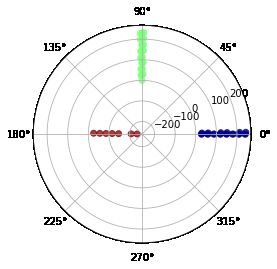
霍夫直线检测回传的结果是极径和极角,每条直线在极坐标空间里表示一个点
可以发现有很多重叠的线,正常来说我们只需要横竖各8条就可以,其实是原图边框线是有一定线宽的,线的两侧包括内侧都会被检测成直线,只要可以连起来且大于设定的阈值就会被检测到。那么我们需要滤除掉一些重复的线:
先选出水平竖直的直线:
# 转为 list
lines_cut = lines.squeeze(1).tolist()
# 排序好进行前后比较
lines_cut = sorted(lines_cut, key=lambda x: x[0])
# 分出水平竖直,这里由于cv的坐标系不同,所以theta为pi/2的线画出来是水平的
h_lines = [l for l in lines_cut if l[0] > 0 and 1.5 <= l[1] < 1.6]
v_lines = [l for l in lines_cut if l[0] > 0 and 0 <= l[1] < 0.1]

# 展示挑选后的结果
lines_cut = np.array(h_lines+v_lines)
ax = plt.subplot(111, projection='polar')
c = ax.scatter(lines_cut[:, 1], lines_cut[:, 0],
               c=lines_cut[:, 1], cmap=plt.cm.jet, alpha=0.75)
plt.show()

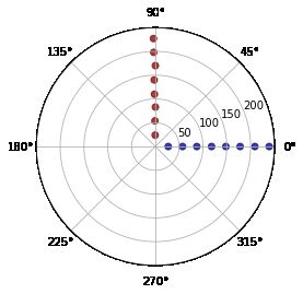
好的,只剩下水平数值的线啦,然后我们剔除多余的线,再利用上面的求解坐标的方法将剩下的线画在空画布上:
h_lines_cut = [h_lines[0]]
v_lines_cut = [v_lines[0]]
# 两线之间rho最小间距
gap = 10
for l in h_lines:
    if l[0]-h_lines_cut[-1][0] > gap:
        h_lines_cut.append(l)
for l in v_lines:
    if l[0]-v_lines_cut[-1][0] > gap:
        v_lines_cut.append(l)
# 重组
lines_cut = np.array(h_lines_cut+v_lines_cut)
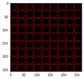
画在空画布上显示:
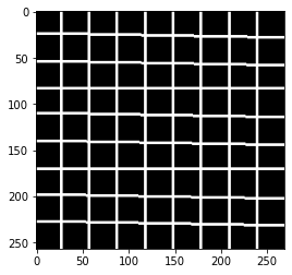
DFS连通域检测+操刀裁剪
现在画出来的线就很舒服啦,然后我们来进行81个宫格的划分,这里我使用的是DFS求连通域,因为每个待裁剪的区域都被白色边界包围,所以就是一个连通域。
通过DFS遍历一遍图像,就可以把所有的连通域找到啦,这么说也很抽象,看过之前推文的小朋友看到下面的实现就会很熟悉啦,当然这个过程也可以用BFS来做喔:
def bfs_maze(src):
    from queue import Queue
    sub_rect = []
    # 标记数组
    vis = np.zeros_like(src)
    direction = [[-1, 0], [0, -1], [1, 0], [0, 1]]
    row, col = src.shape[0], src.shape[1]
    print(row, col)
    # 边界检查
    def check(x, y):
        nonlocal row, col
        return 0 <= x < row and 0 <= y < col
    # dfs
    def dfs(x, y, sp):
        nonlocal src, vis, direction
        # 标记状态
        vis[x][y] = 1
        # 存入临时list
        sp.append((x, y))
        for d in direction:
            nx, ny = x+d[0], y+d[1]
                # 如果下一个点再边界内,而且像素值为0且还没被标记过
                if check(nx, ny) and vis[nx][ny] == 0 and src[nx][ny] == 0:
                    dfs(nx, ny, sp)
    for i in range(row):
        for j in range(col):
            if src[i, j] == 0 and vis[i][j] == 0:
                # 存储连通域内的点
                sp = []
                dfs(i, j, sp)
                # reshape -> (-1,1,2)
                sp = np.array(sp).reshape((len(sp), 1, 2))
                # 寻找最小包围矩形框:将连通域视为一组轮廓
                min_rect = cv.minAreaRect(sp)
                # 得到矩形角点
                rect_points = cv.boxPoints(min_rect).tolist()
                # 计算左上和右下顶点
                sum_t = [sum(a) for a in rect_points]
                tl = rect_points[sum_t.index(min(sum_t))]
                br = rect_points[sum_t.index(max(sum_t))]
                # 不是那种可能是边界的长条形矩形,并且宽度不是很小,处于图像之中则满足要求
                if 5 < br[0]-tl[0] <= src.shape[0]//9*2 \
                        and 5 < br[1]-tl[1] <= src.shape[1]//9*2 \
                        and 0 <= tl[0] < row-5 and 0 <= tl[1] < col-5:
                    sub_rect.append([tl[0], tl[1], br[0], br[1]])
    return sub_rect

sr = bfs_maze(img_copy)
print(len(sr))
# 画出所有的矩形
show_img = np.zeros(img_copy.shape+tuple([3]), dtype=np.uint8)
for r in sr:
    # print(r)
    tlx, tly, brx, bry = r
    # 转int,红色,线宽为1
    cv.rectangle(show_img, (int(tly), int(tlx)),
                 (int(bry), int(brx)), (0, 0, 255), 1)
plt.figure()
plt.imshow(cv.cvtColor(show_img, cv.COLOR_BGR2RGB))
plt.show()

"""
[output]
81
"""
结果来说是有81个满足条件的矩形框,是符合预期的,我们来看看矩形框的分布:
我们已经得到各个矩形框的顶点坐标,如果直接分割,一开始会发现有这样的结果:
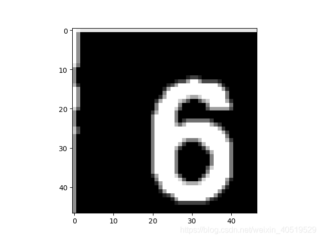
这是由于有一些靠近外框的数字在切割时都可能把最外面的框线包括进去,我们应该进行剔除,具体方法将裁剪区域是向内收缩几个像素:
# 分割
ROI_image = []
# 偏移补偿
x_Shift_Delta = 3
y_Shift_Delta = 3
shift_cor = [x_Shift_Delta, y_Shift_Delta, -x_Shift_Delta, -y_Shift_Delta]
for r in sr:
    tlx, tly, brx, bry = r
    t_img = warped_img[int(tlx)+shift_cor[0]:int(brx)+shift_cor[2],
                       int(tly)+shift_cor[1]:int(bry)+shift_cor[3]]
    ROI_image.append(t_img)
print(len(ROI_image))
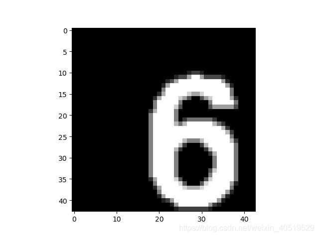
结果就会好一些啦:

我们还会发现尽管收缩的边缘,但是整个数字偏向右下角,显得有点不好(强迫症当场去世,我们可以找到数字6图案的重心然后去迁移到中心,这就好啦~,强迫症当场去试
c e n t e r x = ∑ p i x i ∑ p i center_x=\frac{\sum p_ix_i}{\sum p_i} centerx=∑pi∑pixi
上面是重心计算公式,pi是第i个位置的像素值,xi是第i个位置的x坐标值,那么我们怎么快速来完成呢,这里可以利用矩阵的运算思维,生成一个每一相同行的像素值都是所在行数值的矩阵和一个每以相同列的像素值都是所在列数值的矩阵,与原图像进行相乘,然后求和,再除以原图像像素值的和就OK啦
# 得到系数矩阵
pi_x = np.fromfunction(lambda x, y: x, shape = ROI_image[80].shape, dtype = np.float32)
pi_y = np.fromfunction(lambda x, y: y, shape = ROI_image[80].shape, dtype = np.float32)

然后我们来计算重心:
centroid_y = np.sum(pi_y*ROI_image[idx]) / np.sum(ROI_image[idx])
centroid_x = np.sum(pi_x*ROI_image[idx]) / np.sum(ROI_image[idx])
为了后面的分类,我们应该把所有切割完的数字图像归一到相同的大小,所以我这里采用的是先填充边缘然后再resize的方法
组合成迁移到图像中心的函数:
def shift2center(img,trow,tcol):
    """
    shift the cut number img to center
    args:
    img: src img
    trow:target_row length for result img
    tcol:target_col length for result img
    return: shift2center img
    """
    row,col = img.shape
    pi_x = np.fromfunction(lambda x, y: x, shape = img.shape, dtype = np.float32)
    pi_y = np.fromfunction(lambda x, y: y, shape = img.shape, dtype = np.float32)
    # 判断是否是一些没有数字的空格,即大部分是灰度值为0的像素
    if np.sum(img) > row*col*0.1*255:
        centroid_y = np.sum(pi_y * img) / np.sum(img)
        centroid_x = np.sum(pi_x * img) / np.sum(img)
    else:
        return np.zeros((trow, tcol))
    xc,yc = int(centroid_x), int(centroid_y)
    #print('center coordinates: ',xc,yc)
    # x方向的补偿长度
    delta_x = 0
    # 是否补偿标记
    flag_x, flag_y = 0, 0
    if xc > row - xc:
        flag_x = 1
        t_img = np.concatenate((img, np.zeros((2 * xc - row,col))), axis=0)
        delta_x = 2 * xc-row
    elif xc < row - xc:
        flag_x=1
        t_img = np.concatenate((np.zeros((row - 2 * xc,col)), img),axis = 0)
        delta_x = row - 2 * xc
    if yc > col - yc:
        flag_y = 1
        if delta_x > 0:
            # 如果x方向有补偿,则生成的填充矩阵x方向的长度要改变为 row+delta_x
            t_img = np.concatenate((t_img,np.zeros((row + delta_x, 2 * yc - col))), axis = 1)
        else:
            t_img = np.concatenate((img,np.zeros((row + delta_x, 2 * yc - col))), axis = 1)
    elif yc < col - yc:
        flag_y = 1
        if delta_x > 0:
            t_img = np.concatenate((np.zeros((row + delta_x, col - 2 * yc)), t_img), axis = 1)
        else:
            t_img = np.concatenate((np.zeros((row + delta_x, col - 2 * yc)), img), axis = 1)
    # 不需要补偿
    if flag_x == 0 and flag_y == 0:
        t_img = img
    # resize到目标大小并且二值
    t_img = cv.resize(t_img, (trow, tcol))
    ret, t_img = cv.threshold(t_img.astype(np.uint8), 127, 255, cv.THRESH_OTSU)
    return t_img
我们来看看结果:

还是不错滴,处于图像中间了~
我们来看看其他数字的情况:
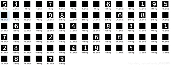
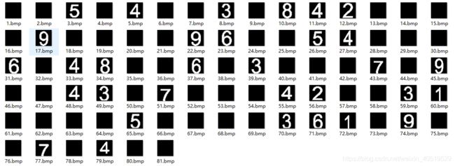
总结
基本符合预期,没有奇奇怪怪的边框混入
本次推文小刀耗时两天多,大部分时间是在阅读函数文档和更改参数并且发现解决一些可能的问题,这里我的方法也不是完美的,也会有可能出现一些乱入情况,需要根据情况调制参数。某些过程里我可能采取了一些较为麻烦的方法,如果有更好的方法欢迎推荐学习。
我要去干饭了………………

Reference
[1] 数独项目第二弹:图像处理pian