阿里天池学习赛-金融风控-贷款违约预测

1 赛题理解

项目地址：
https://github.com/datawhalechina/team-learning-data-mining/tree/master/FinancialRiskControl

比赛地址：
https://tianchi.aliyun.com/competition/entrance/531830/introduction

1.1 赛题数据

赛题以预测金融风险为任务，数据集报名后可见并可下载，该数据来自某信贷平台的贷款记录，总数据量超过120w，包含47列变量信息，其中15列为匿名变量。为了保证比赛的公平性，将会从中抽取80万条作为训练集，20万条作为测试集A，20万条作为测试集B，同时会对employmentTitle、purpose、postCode和title等信息进行脱敏。

字段如下：

Field	Description
id 为贷款清单分配的唯一信用证标识
loanAmnt	贷款金额
term	贷款期限（year）
interestRate	贷款利率
installment	分期付款金额
grade	贷款等级
subGrade	贷款等级之子级
employmentTitle	就业职称
employmentLength	就业年限（年）
homeOwnership	借款人在登记时提供的房屋所有权状况
annualIncome	年收入
verificationStatus	验证状态
issueDate	贷款发放的月份
purpose	借款人在贷款申请时的贷款用途类别
postCode	借款人在贷款申请中提供的邮政编码的前3位数字
regionCode	地区编码
dti	债务收入比
delinquency_2years	借款人过去2年信用档案中逾期30天以上的违约事件数
ficoRangeLow	借款人在贷款发放时的fico所属的下限范围
ficoRangeHigh	借款人在贷款发放时的fico所属的上限范围
openAcc	借款人信用档案中未结信用额度的数量
pubRec	贬损公共记录的数量
pubRecBankruptcies	公开记录清除的数量
revolBal	信贷周转余额合计
revolUtil	循环额度利用率，或借款人使用的相对于所有可用循环信贷的信贷金额
totalAcc	借款人信用档案中当前的信用额度总数
initialListStatus	贷款的初始列表状态
applicationType	表明贷款是个人申请还是与两个共同借款人的联合申请
earliesCreditLine	借款人最早报告的信用额度开立的月份
title	借款人提供的贷款名称
policyCode	公开可用的策略_代码=1新产品不公开可用的策略_代码=2
n系列匿名特征	匿名特征n0-n14，为一些贷款人行为计数特征的处理

1.2 评测标准

提交结果为每个测试样本是1的概率，也就是y为1的概率。评价方法为AUC评估模型效果

2 探索性分析（EDA）

探索性分析可以让我们更好了解数据以及数据之间的关系，让我们在数据清洗和建模的时候能够更加顺利。

2.1 初窥数据

首先导入数据并且大致看一下数据

test = pd.read_csv("./testA.csv")
train = pd.read_csv("./train.csv")
train.drop("id", axis= 1,inplace = True)
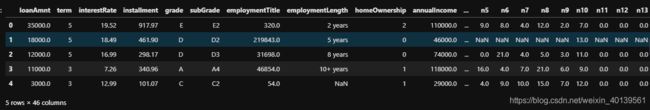
train.head()
train.info(verbose = True)
train.describe()

<class 'pandas.core.frame.DataFrame'>
RangeIndex: 800000 entries, 0 to 799999
Data columns (total 46 columns):
loanAmnt              800000 non-null float64
term                  800000 non-null int64
interestRate          800000 non-null float64
installment           800000 non-null float64
grade                 800000 non-null object
subGrade              800000 non-null object
employmentTitle       799999 non-null float64
employmentLength      753201 non-null object
homeOwnership         800000 non-null int64
annualIncome          800000 non-null float64
verificationStatus    800000 non-null int64
issueDate             800000 non-null object
isDefault             800000 non-null int64
purpose               800000 non-null int64
postCode              799999 non-null float64
regionCode            800000 non-null int64
dti                   799761 non-null float64
delinquency_2years    800000 non-null float64
ficoRangeLow          800000 non-null float64
ficoRangeHigh         800000 non-null float64
openAcc               800000 non-null float64
pubRec                800000 non-null float64
pubRecBankruptcies    799595 non-null float64
revolBal              800000 non-null float64
revolUtil             799469 non-null float64
totalAcc              800000 non-null float64
initialListStatus     800000 non-null int64
applicationType       800000 non-null int64
earliesCreditLine     800000 non-null object
title                 799999 non-null float64
policyCode            800000 non-null float64
n0                    759730 non-null float64
n1                    759730 non-null float64
n2                    759730 non-null float64
n2.1                  759730 non-null float64
n4                    766761 non-null float64
n5                    759730 non-null float64
n6                    759730 non-null float64
n7                    759730 non-null float64
n8                    759729 non-null float64
n9                    759730 non-null float64
n10                   766761 non-null float64
n11                   730248 non-null float64
n12                   759730 non-null float64
n13                   759730 non-null float64
n14                   759730 non-null float64
dtypes: float64(33), int64(8), object(5)
memory usage: 280.8+ MB

发现数据的类型主要既有数值型也有分类变量，并且有不少变量中存在缺失值。

#正负样本
plt.hist(train['isDefault'])
plt.title("positive vs negative")
plt.show()

可以看到负样本比正样本多很多，这也是金融风控模型评估的中常见的现象，毕竟大多数的人还是不会拖欠贷款的。

2.2 查看缺失值占比

#缺失值占比
missing_val = train.isnull().sum()/train.shape[0]
missing_val[missing_val >0].sort_values().plot.bar()

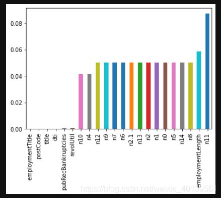
缺失值最多的变量是n11，大概占9%，但是还不算特别多，因此这个变量还是可以保留的
一般缺失值的办法有很多，如果缺失值很多的话可以选择删除变量，否则可以根据适当的方法进行填充，一般有平均值填充法，众数填充或者随机森林填充等，可以根据具体情况选择。

2.3 数值型变量

稍微深入查看数值型变量

2.3.1 数据分布

numerical_cols = []
for col in train.columns:
    if train[col].dtype != object:
        numerical_cols.append(col)  #数值列
numerical_cols.remove("isDefault")
f,ax = plt.subplots(len(numerical_cols)//4,4,figsize = (15,60))
for i, col in enumerate(numerical_cols):
    sns.distplot(train[col], ax = ax[i//4,i%4])

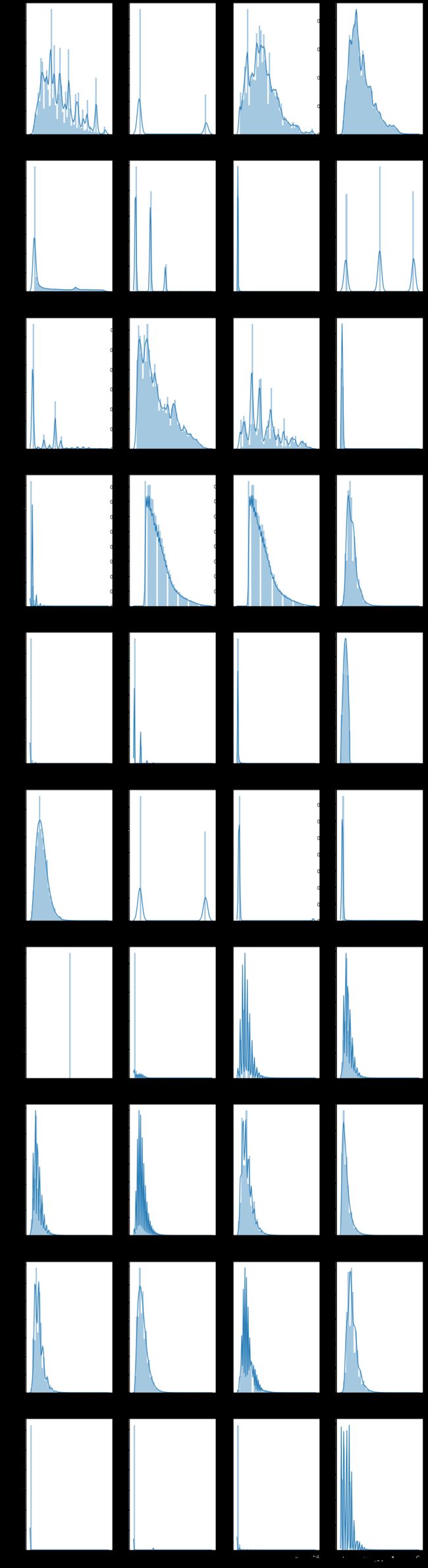
这里可以看出几点：

• 大部分数据呈现出右偏趋势，说明数据较大的可能是异常值
• policyCode 只有一个取值，因此这个变量对于预测不会起到任何作用，可以删除；initialListstatus是一个二分类变量；n2 和n2.1有非常相似的分布，可能是重复列

2.3.2 变量关系

用热力图查看各变量之间的关系，比较值观

f, ax = plt.subplots(1,1, figsize = (20,20))
cor = train[numerical_cols].corr()
sns.heatmap(cor, annot = True, linewidth = 0.2, linecolor = "white", ax = ax, fmt =".1g" )

从这个图中能看到有一些变量有很强的相关性：

• loanAmnt 和installment 相关性为1， 这两个变量一个是贷款总额，一个是分期付款金额，因此这两者是会有很强的想关性

• ficoRangeLow he ficoRangeHigh 相关性为1，这两个是fico的上下限，因此也肯定有很强的相关性

• n2和n2.1也有强相关性，根据之前的分布图来看，这两列基本可以确定是重复列，可以删除其中一列

• n1 n2 n4 n5 n7 n9 n10正相关关系较强

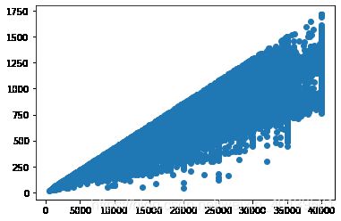
• installment(Y) 和 loanAmnt (X)的关系图

plt.scatter(train['loanAmnt'],train['installment'])

• ficoRangeLow he ficoRangeHigh 关系图

 plt.scatter(train['ficoRangeLow'],train['ficoRangeHigh'])

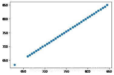
这两个变量就是线性关系，因此也可以删除其中一个

2.4 离散变量

离散变量数不能直接用来建模的，必须通过一定的处理变成数值之后再放进模型，方法有很多。可以直接映射，也有one-hot Encoding, Target Encoding等编码方式。在风控模型中还会常用到分箱的方法赋值。

2.4.1 数据分布

• Grade

train['grade'].value_counts().sort_index().plot.bar()

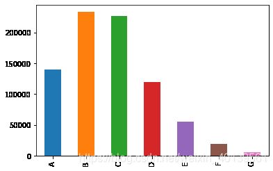
可以直接映射转化

• subGrade

train['subGrade'].value_counts().sort_index().plot.bar(figsize=(15,5))

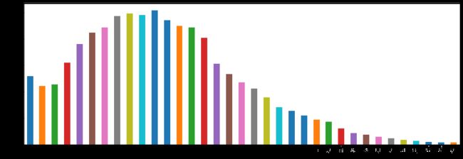
还是可以考虑映射，或者分箱

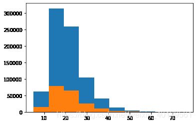
• issueDate
  日期变量，贷款发放时间，转换为离数据集最早的发放时间的天数差

def transform_issueDate(df):
    df['issueDate'] = pd.to_datetime(df['issueDate'],format='%Y-%m-%d')
    startdate = datetime.datetime.strptime('2007-06-01', '%Y-%m-%d')
    df['issueDateDT'] = df['issueDate'].apply(lambda x: x-startdate).dt.days
    return df
train = transform_issueDate(train)
test = transform_issueDate(test)
plt.hist(train['issueDateDT'],label = "train")
plt.hist(test['issueDateDT'], label = "test")

• earliesCreditLine_Year
  贷款人最早报告的信用额度的时间
  转化为在距离2020的年数

def transform_earliesCreditLine(df):
    df['earliesCreditLine_Year'] = df['earliesCreditLine'].apply(lambda x: 2020-int(x[-4:]))
    return df
train =  transform_earliesCreditLine(train)
test =  transform_earliesCreditLine(test)
plt.hist(train['earliesCreditLine_Year'],label = "train")
plt.hist(test['earliesCreditLine_Year'],label = "test")

2.5 正负样本的数据差异

把数据集按正负样本分成两份，查看变量的分布差异

train_positve = train[train['isDefault'] == 1]
train_negative = train[train['isDefault'] != 1]
f, ax = plt.subplots(len(numerical_cols),2,figsize = (10,80))
for i,col in enumerate(numerical_cols):
    sns.distplot(train_positve[col],ax = ax[i,0],color = "blue")
    ax[i,0].set_title("positive")
    sns.distplot(train_negative[col],ax = ax[i,1],color = 'red')
    ax[i,1].set_title("negative")
plt.subplots_adjust(hspace = 1)

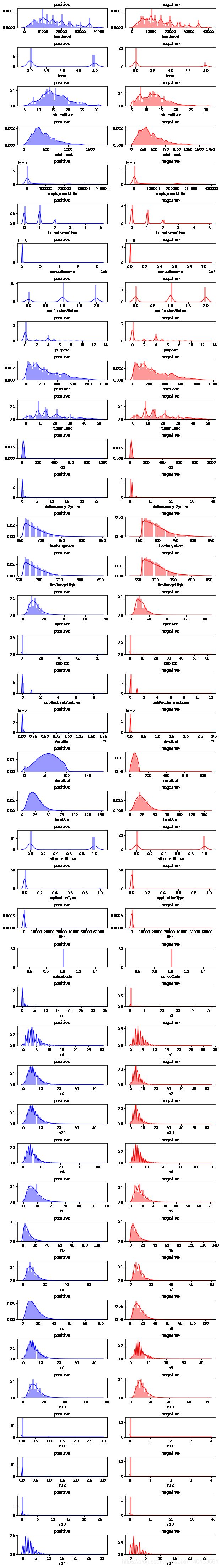
总体的分布差异不大，revolUtil的差别较大

3 特征工程

特征筛选是机器学习里面比较重要的一个环节，特征工程大致包括以下步骤：

• 数据预处理
• 异常值处理
• 数据分箱
• 特征衍生
• 数据编码
• 特征选择

3.1 数据预处理

数据预处理大致包括以下三个方面：

• 缺失值处理
• 时间格式处理
• 对象类型特征转换到数值

3.1.1 缺失值处理

在上一步我们查看了缺失值，有不少变量中存在缺失值，并且可以看到n10和n4缺失值的数量是一样的，除了n10，n4和n11之外的其他匿名变量的缺失值数量也是一样的，所以很有可能这些缺失值在这些变量中同时缺失
以下验证我们的猜想

is_null_index = train['n10'].isnull()
for col in train.columns:
    if train[col][is_null_index].notnull().sum() == 0:
        print(col)
        
n0
n1
n2
n2.1
n4
n5
n6
n7
n8
n9
n10
n11
n12
n13
n14

is_null_index = train['n1'].isnull()
for col in train.columns:
    if train[col][is_null_index].notnull().sum() == 0:
        print(col)
        
n0
n1
n2
n5
n6
n7
n8
n9
n11
n12
n13
n14

以上结果可以看出，n10缺失的行，其他匿名变量也全部缺失；n1缺失的行，除了n10和n4也全部缺失。因此推测这些匿名变量是有一定关联性的：

• n10缺失，则匿名变量均缺失；
• n1缺失，则除n10和n4以外的所有匿名变量均缺失；

这样看来匿名变量的缺失不应该填充，应该当作一个值丢进模型。
EmploymentLength这个变量的缺失值也比较多

3.1.2 时间格式处理

这个数据集一共有两个时间变量，在EDA的时候已经顺便处理了

3.1.3 对象类型特征转换到数值

对象类型特征有“grade",“subGrade” 和 ”employmentLength“

• "grade"和”subGrade“都是表示贷款等级的特征，因此应该是有一定的顺序的，比如A>B，A1>A2之类，因此可以直接映射成数值，这种方法和Label Encoding 是一样的。

for colname in ['grade',"subGrade"]
    unique_num = train.append(test)[colnamee].nunique()
    unuque_val = sorted(train.append(test)[colname].unique())
    for data in [train,test]:
        map_dict = {
     x:y for x,y in zip(unuque_val,range(unique_num))}
        data[colname] = data[colname].map(map_dict)

• “employmentLength”

train['employmentLength'].unique()

array(['2 years', '5 years', '8 years', '10+ years', nan, '7 years',
       '9 years', '1 year', '3 years', '< 1 year', '4 years', '6 years'],
      dtype=object)

把数字后面的years去掉并且把10+改成10，<1改成0

for data in [train,test]:
    data['employmentLength'].replace("< 1 year", "0 year", inplace=True)
    data['employmentLength'].replace("10+ years", "10 years", inplace=True)
    data['employmentLength'] = data['employmentLength'].apply(lambda x: int(str(x).split()[0]) if pd.notnull(x) else x)

3.2 异常值处理

异常值的存在很可能会影响模型的最终结果，但是当我们发现异常值的时候也不能马上就删除，应该先看看这个异常值是不是有特殊原因造成的，特别是在金融风控问题中，异常值的出现往往是存在意义的。

此处打算先不作异常值处理，二十

3.3 数据分箱

• L特征分箱的目的：
  从模型效果上来看，特征分箱主要是为了降低变量的复杂性，减少变量噪音对模型的影响，提高自变量和因变量的相关度。从而使模型更加稳定。
• 数据分桶的对象：
  • 将连续变量离散化
  • 将多状态的离散变量合并成少状态
• 分箱的原因：
  数据的特征内的值跨度可能比较大，对有监督和无监督中如k-均值聚类它使用欧氏距离作为相似度函数来测量数据点之间的相似度。都会造成大吃小的影响，其中一种解决方法是对计数值进行区间量化即数据分桶也叫做数据分箱，然后使用量化后的结果。
• 分箱的优点：
  • 处理缺失值：当数据源可能存在缺失值，此时可以把null单独作为一个分箱。
  • 处理异常值：当数据中存在离群点时，可以把其通过分箱离散化处理，从而提高变量的鲁棒性（抗干扰能力）。例如，age若出现200这种异常值，可分入“age > 60”这个分箱里，排除影响。
  • 业务解释性：我们习惯于线性判断变量的作用，当x越来越大，y就越来越大。但实际x与y之间经常存在着非线性关系，此时可经过WOE变换。
• 特别要注意一下分箱的基本原则：

（1）最小分箱占比不低于5%
（2）箱内不能全部是好客户
（3）连续箱单调

python暂时没找到卡方分箱的包，按照自己的理解手写了一个

import numpy as np
class ChiMerge():
    def __init__(self,df,col_name,target):
        self.num_bins = df[col_name].nunique() 
        self.sorted_df = df.sort_values(by = col_name)[[target,col_name]]
        self.target = target
        self.unique_val =  np.sort(df[col_name].unique())
        self.col_name = col_name
        self.reverse = 1
        self.shape = df.shape[0]
        
    def check_max_and_min_bin(self,to_merge_df):
        max_bin = to_merge_df[self.col_name].value_counts().values[0]
        
        min_bin = to_merge_df[self.col_name].value_counts().values[-1]

        return max_bin/self.shape, min_bin/self.shape   
    
    def cal_Chi2(self,bin1,bin2, epsilon = 1e-8):
        #计算单个两个箱体的卡方值，加入epsilon为了防止除0错误
        
        bins = bin1.append(bin2)
        total = bins.shape[0]
        positive_rate = bins[self.target].sum()/total
        negative_rate = 1- positive_rate
        
        chi2_val = (bin1[self.target].sum() - positive_rate * bin1.shape[0])**2/(positive_rate * bin1.shape[0] + epsilon) +\
        (bin2[self.target].sum() - positive_rate * bin2.shape[0])**2/(positive_rate * bin2.shape[0] +epsilon) +\
        (bin1.shape[0] - bin1[self.target].sum() - negative_rate * bin1.shape[0])**2/(negative_rate * bin1.shape[0] + epsilon)+\
        (bin2.shape[0] - bin2[self.target].sum() - negative_rate * bin2.shape[0])**2/(negative_rate * bin2.shape[0] + epsilon)
        
        return chi2_val
    
    def calculate_every_Chi2(self):
        
        chi2_list = []
        if self.reverse ==1:
            # 如果数值较多的时候可能会出现很多卡方为0的箱，为了减少次数，两头循坏，避免全列表遍历
            # 水平较低，想暂时使用这个方法减少分箱时间
            for i in range(self.num_bins - 1):
                chi2  = self.cal_Chi2(self.sorted_df[self.sorted_df[self.col_name]==self.unique_val[i]],self.sorted_df[self.sorted_df[self.col_name]==self.unique_val[i+1]])
                chi2_list.append(chi2)
                if chi2 ==0:
                    break
        else:
            for i in range(self.num_bins - 1,0,self.reverse):
                chi2  = self.cal_Chi2(self.sorted_df[self.sorted_df[self.col_name]==self.unique_val[i]],self.sorted_df[self.sorted_df[self.col_name]==self.unique_val[i+1]])
                chi2_list.append(chi2)
                if chi2 ==0:
                    break
                    
            
        self.reverse = self.reverse * (-1)
        
        return chi2_list
    

    def chi2Merge(self,chi2_val):

        max_bin,min_bin = self.check_max_and_min_bin(self.sorted_df)
        
        if max_bin>0.95:
            print("The max bin has more than 95% of samples")
            return self.sorted_df
        # 先初次判断，如果初始数据已经有箱体过大的情况，无法分箱
            
        chi2_list = [0]
        while self.num_bins > 5 and min(chi2_list) < chi2_val: 
            
            remove_flag = True
            chi2_list = self.calculate_every_Chi2()
            unique_val = self.unique_val
            
            while remove_flag:
                to_merge = np.argmin(chi2_list)
                to_merge_df = self.sorted_df
                to_merge_df[self.col_name][to_merge_df[self.col_name] == unique_val[to_merge]] = unique_val[to_merge + 1]
                max_bin,min_bin = self.check_max_and_min_bin(to_merge_df)
                if max_bin > 0.95:
                    chi2_list.pop(to_merge)
                    unique_val.pop(to_merge)
                else:
                    remove_flag = False
                    self.unique_val = unique_val
                    
            self.sorted_df[self.col_name][self.sorted_df[self.col_name] == self.unique_val[to_merge]] = self.unique_val[to_merge + 1]
            self.unique_val =  np.sort(self.sorted_df[self.col_name].unique())
            self.num_bins -=1
            if self.num_bins%1000 == 0:
                print(self.num_bins)
        _,min_bin = self.check_max_and_min_bin(self.sorted_df)
        if min_bin < 0.05:
            print("too small bin")

在初始值较多的特征上使用的话速度比较慢，而且分箱结果不太好，打算之后再尝试改进或者使用其他方法。

3.4 数据编码

编码就是把一些离散的变量变成能够表示特征间关系的的数值放入模型，常用的方法有:

• Label Encoding
  即类似{A=1,B=2}的映射
• One-Hot Encoding
  生成稀疏矩阵，比如有A,B,C三类，分别表示为[0,0,1] [0,1,0]和 [1,0,0]
• Target Encoding
  把target的均值赋给变量，比如：

target	feature
1	A
1	A
1	A
0	A
1	B
1	B
0	B
0	B

取值为A时，有三个target是1，一个是0，因此A = 3/4=0.75
同理 B= 2/4 = 0.5
这个方法的缺点是容易过拟合，因此一般会使用交叉验证或者添加噪音的方式去编码，我们这里的编码使用target encoding

class KFoldTargetEncoderTrain(base.BaseEstimator, base.TransformerMixin):

    def __init__(self, colnames,targetName,n_fold=5,verbosity=True,discardOriginal_col=False):

        self.colnames = colnames
        self.targetName = targetName
        self.n_fold = n_fold
        self.verbosity = verbosity
        self.discardOriginal_col = discardOriginal_col

    def fit(self, X, y=None):
        return self


    def transform(self,X):

        assert(type(self.targetName) == str)
        assert(type(self.colnames) == str)
        assert(self.colnames in X.columns)
        assert(self.targetName in X.columns)

        mean_of_target = X[self.targetName].mean()
        kf = KFold(n_splits = self.n_fold, shuffle = False)



        col_mean_name = self.colnames + '_' + 'Kfold_Target_Enc'
        X[col_mean_name] = np.nan

        for tr_ind, val_ind in kf.split(X):
            X_tr, X_val = X.iloc[tr_ind], X.iloc[val_ind]
#             print(tr_ind,val_ind)
            X.loc[X.index[val_ind], col_mean_name] = X_val[self.colnames].map(X_tr.groupby(self.colnames)[self.targetName].mean())

        X[col_mean_name].fillna(mean_of_target, inplace = True)

        if self.verbosity:

            encoded_feature = X[col_mean_name].values
            print('Correlation between the new feature, {} and, {} is {}.'.format(col_mean_name,
                                                                                      self.targetName,
                                                                                      np.corrcoef(X[self.targetName].values, encoded_feature)[0][1]))
        if self.discardOriginal_col:
            X = X.drop(self.colnames, axis=1)
            
        return X
    
class KFoldTargetEncoderTest(base.BaseEstimator, base.TransformerMixin):
    
    def __init__(self,train,colNames,encodedName):
        
        self.train = train
        self.colNames = colNames
        self.encodedName = encodedName
        
        
    def fit(self, X, y=None):
        return self

    def transform(self,X):


        mean = self.train[[self.colNames,self.encodedName]].groupby(self.colNames).mean().reset_index() 
        
        dd = {
     }
        for index, row in mean.iterrows():
            dd[row[self.colNames]] = row[self.encodedName]

        
        X[self.encodedName] = X[self.colNames]
        X = X.replace({
     self.encodedName: dd})

        return X

对’purpose’,“verificationStatus”, “regionCode”,“grade”,"subGrade"五个变量进行target encoding

for colname in ['purpose',"verificationStatus", "regionCode"，"grade"，"subGrade"]:
    targetc = KFoldTargetEncoderTrain(colname,'isDefault',n_fold=5)
    train = targetc.fit_transform(train)
    test_targetc  = KFoldTargetEncoderTest(train,colname,colname + '_' + 'Kfold_Target_Enc')
    test = test_targetc.fit_transform(test)

3.5 特征衍生

3.11 里提到了匿名变量里缺失值可能是某种原因造成的，分成以下三类缺失查看正负样本比

1. 只有n11缺失
2. 除了n4和n10之外都缺失
3. 全部缺失
4. 无缺失

for data in [train,test]:
    data['extra_col1'] = 3
    data['extra_col1'].loc[data['n10'].isnull()] = 1
    data['extra_col1'].loc[data['n1'].isnull() & data['n10'].notnull()] = 2
    data['extra_col1'].loc[data['n11'].isnull() & data['n1'].notnull()] = 4
 for i in range(1,5):
    print(train[train['extra_col1']==i]['isDefault'].sum()/train[train['extra_col1']==i]['isDefault'].count())

0.14362646288997863
0.17678850803584129
0.19927476692849552
0.27382809850078016

以上说明缺失值的程度似乎对正负样本的比例有影响，因此我们可以衍生一个这样的变量尽管他的关系不一定是线性的(后续可以进行Target Encoding)。

LA_ration (loanAmnt / annualIncome)

3.5 特征筛选

特征筛选目的是在不牺牲模型效果的情况下减少模型和训练时间，由于此处数据集并不算特别大，暂时先不做特征筛选，如果后面有需要再回来补充这一步骤。

4 建模及调参

之前做了这么多准备工作，最后的目的还是为了输出结果，这一步我们可以开始建立模型，并且根据评价指标不断优化模型

这次建模打算先用机器学习建模神器Xgboost，使用的是sklearn的接口，先导入可能会用到的包

from xgboost import XGBClassifier
from sklearn.model_selection import train_test_split,KFold
from sklearn.metrics import auc, roc_curve
from xgboost import plot_importance
from sklearn.metrics import auc, roc_curve
from sklearn.model_selection import GridSearchCV,RandomizedSearchCV

4.1 Baseline

target = train['isDefault']
train_X = train.drop("isDefault", axis=1)
#切分训练和检验集
X_train,X_test,y_train,y_test = train_test_split(train_X, target,test_size = 0.2, random_state = 0)

随手设置一些参数：

def XGB():
    model =  XGBClassifier(learning_rate=0.1,
                              n_estimators=600,             
                              max_depth=5,                
                              min_child_weight=5,      
                              gamma=1,                 
                              subsample=0.8,        
                              random_state=27,              
                              verbosity= 1,                   
                              nthread=-1
                          )
    return model
    

具体的xgboost 参数设置可以参考官网

%%time
model = XGB()
model.fit(X_train, y_train, eval_set = [(X_train,y_train),(X_test,y_test)],eval_metric="auc")
result = model.evals_result()


pre = model.predict_proba(X_train)[:,1]
fpr, tpr, thresholds = roc_curve(y_train, pre)
score = auc(fpr, tpr)

f,[ax1,ax2] = plt.subplots(2,1,figsize = (7,15))

ax1.plot([i for i in range(1,600+1)],result['validation_0']['auc'])
ax1.plot([i for i in range(1,600+1)],result['validation_1']['auc'])
ax2.set_xlim(0,1)
ax2.set_ylim(0,1)
ax2.plot(fpr,tpr,label = "AUC = {:.3f}".format(score))
ax2.plot([0,1],[0,1],linestyle = "--")
plt.legend()

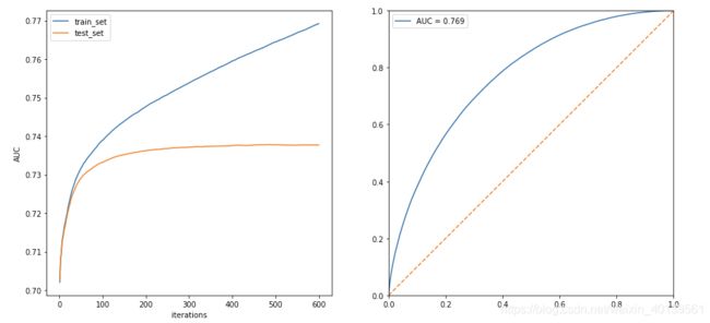
左图表示随着迭代次数，训练集和测试集的AUC变化，可以看到大概在200次迭代以后测试集的auc变化就已经很小了，因此后续可以把n_estimator设置在200-300之前以减少训练时间

4.2 调参

有了baseline 之后我们可以根据基础模型对模型参数进行优化。
由于Xgboost参数较多，而且运行的速度比较慢，如果直接使用网格搜索可能要耗费几天时间，因此我们按一个参数一个参数调。

在定义以下基准模型
model = XGBClassifier(
    learning_rate=0.1,
    n_estimators=300,             
    max_depth=5,                 
    min_child_weight=6,        
    gamma=1,                    
    subsample=0.8,   
    scale_pos_weight=4,          
    random_state=27,                 
    verbosity= 1,                   
    nthread=-1 
)

4.2.1 max_depth

这个参数决定最大深度

param_grid = {
     
	"max_depth":[i for i in range(3, 11)]
}
xgb_grid = GridSearchCV(
	model,
	param_grid = param_grid, 
	scoring= #"roc_auc", "这次评价标准的auc"
	verbose=True, #"输出过程"
	cv=5, #"5折检验"
	n_jobs=-1 #"使用所有CPU"
	) 
xgb_grid.best_param_
# 5

4.2.2min_child_weight

最小叶子节点权重和，如果在一次分裂中，叶子节点上所有样本的权重和小于min_child_weight則停止分裂，能够有效的防止过拟合，防止学到特殊样本。

param_grid = {
     
	"min_child_weight":[i for i in range(3, 11)]
}
xgb_grid = GridSearchCV(
	model,
	param_grid = param_grid, 
	scoring= #"roc_auc", "这次评价标准的auc"
	verbose=True, #"输出过程"
	cv=5, #"5折检验"
	n_jobs=-1 #"使用所有CPU"
	) 
xgb_grid.best_param_
# 6

4.2.3 subsample

param_grid = {
     
	"subsampele":[i*0.1 for i in range(3, 11)]
}
xgb_grid = GridSearchCV(
	model,
	param_grid = param_grid, 
	scoring= #"roc_auc", "这次评价标准的auc"
	verbose=True, #"输出过程"
	cv=5, #"5折检验"
	n_jobs=-1 #"使用所有CPU"
	) 
xgb_grid.best_param_
# 0.6

4.3 更新模型

使用调整后的参数再次进行检验

def XGB():
    model =  XGBClassifier(learning_rate=0.1,
                              n_estimators=600,             
                              max_depth=5,                
                              min_child_weight=6,      
                              gamma=1,                 
                              subsample=0.6,        
                              random_state=27,              
                              verbosity= 1,                   
                              nthread=-1
                          )
    return model
    
%%time
model = XGB()
model.fit(X_train, y_train)
pre = model.predict_proba(X_test)[:,1]
fpr, tpr, thresholds = roc_curve(y_test, pre)
score = auc(fpr, tpr)
print(score)
#0.7373661712901491

4.4 预测结果并提交

使用更新好的模型提交结果看看最终评分怎样

test= test[train_X.columns]
pre = model.predict_proba(test)[:,1]
pd.DataFrame({
     'isDefault':pre},index=test.index).reset_index().rename(columns={
     "index":"id"}).to_csv('submit.csv', index=0)

线上的AUC得分是0.7337，目前大概排在前50

5 模型融合

模型融合大概有三种：stacking,bagging,blending和boosting
由于xgboost本身就已经是基于boosting的算法，而随机森林是基于bagging的算法，因此这两种将不会在这使用了，主要还是通过blending和stacking来融合模型

5.1 stacking\blending详解

• stacking 将若干基学习器获得的预测结果，将预测结果作为新的训练集来训练一个学习器。但是由于直接由多个基学习器获得结果直接带入模型中，容易导致过拟合。所以在使用多个基模型进行预测的时候，可以考虑使用K折验证，防止过拟合。

• blending 与stacking不同，blending是将预测的值作为新的特征和原特征合并，构成新的特征值，用于预测。为了防止过拟合，将数据分为两部分d1、d2，使用d1的数据作为训练集，d2数据作为测试集。预测得到的数据作为新特征使用d2的数据作为训练集结合新特征，预测测试集结果。

• Blending与stacking的不同

  • stacking
    stacking中由于两层使用的数据不同，所以可以避免信息泄露的问题。
    在组队竞赛的过程中，不需要给队友分享自己的随机种子。
  • Blending
    由于blending对将数据划分为两个部分，在最后预测时有部分数据信息将被忽略。
    同时在使用第二层数据时可能会因为第二层数据较少产生过拟合现象。

5.1 stacking 代码

使用之前的训练的lgb和xgb模型作为基分类器，逻辑回归作为目标分类器做stacking

from mlxtend.classifier import StackingClassifier
sclf = StackingClassifier(classifiers=[lgb_model,xgb_model], 
                          meta_classifier=LR,
                         use_probas=True,
                         verbose= 1)
sclf.fit(X_train,y_train)
pre =sclf.predict_proba(X_test)[:,1]
fpr, tpr, thresholds = roc_curve(y_test, pre)
score = auc(fpr, tpr)
print(score)
#0.7390504896093062

最后提交测试结果，得分为0.7347