问题综述
About Company
Dream Housing Finance company deals in all home loans. They have presence across all urban, semi urban and rural areas. Customer first apply for home loan after that company validates the customer eligibility for loan.
Problem
Company wants to automate the loan eligibility process (real time) based on customer detail provided while filling online application form. These details are Gender, Marital Status, Education, Number of Dependents, Income, Loan Amount, Credit History and others. To automate this process, they have given a problem to identify the customers segments, those are eligible for loan amount so that they can specifically target these customers. Here they have provided a partial data set.
用已知数据预测某人是否可以得到贷款,这是一个分类问题,我们可以用logistic regression,决策数和随机森林等模型建模。
数据连接:https://github.com/Paliking/ML_examples/tree/master/LoanPrediction
理解数据
VARIABLE DESCRIPTIONS:
Variable                    Description
Loan_ID                     ID
Gender                      性别
Married                     是否结婚(Y/N)
Dependents                  家属人数
Education                   是否是大学毕业生
Self_Employed               自雇人士(Y/N)
ApplicantIncome             申报收入
CoapplicantIncome           家庭收入
LoanAmount                  贷款金额
Loan_Amount_Term            贷款天数
Credit_History              信用记录
Property_Area               房产位置
Loan_Status                 是否批准贷款(Y/N)
观察数据特征
对数据的观察是为了更好的了解数据,判断出有用的变量,也为数据预处理提供依据。
数值观察
先读取数据集
# -*- coding: utf-8 -*-
%matplotlib inline
plt.rcParams['font.sans-serif']=['SimHei']
plt.rcParams['axes.unicode_minus']=False#防止作图中文乱码
import pandas as pd
import numpy as np
import matplotlib as plt
df = pd.read_csv(r'C:\Users\Administrator\Desktop\train_u6lujuX_CVtuZ9i.csv',index_col=0)
总览数据集
df.shape
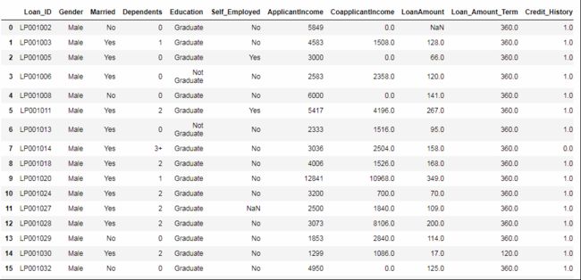
观察前20条数据
df.head(20)
可以使用info跟能看到全局
df.info()

用describe描述统计数据
df.describe()

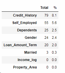
看看空值

total =df.isnull().sum().sort_values(ascending=False)
percent_1 =df.isnull().sum()/df.isnull().count()*100
percent_2 = (round(percent_1, 1)).sort_values(ascending=False)
missing_data = pd.concat([total, percent_2], axis=1, keys=['Total', '%'])
missing_data.head(8)

对于非数值变量我们可以用value_counts来计数
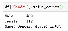
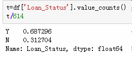
约有69%的人得到了贷款
从统计结果我们可以看到:
1,7个变量存在空值。
2,84%的人有信用记录,约有69%的人得到了贷款。
3,从分位数看申请人收入情况,大致情况没有异常;从最大值来看申报收入和家庭收入都有离群值
申请者各属性分布
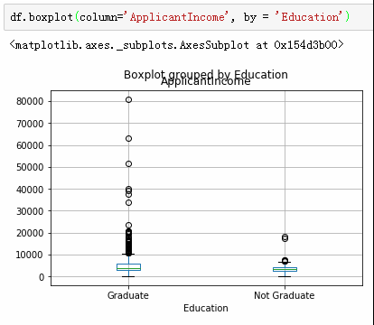
申报收入箱线图
df.boxplot(column='ApplicantIncome')

极端值过多了,这种现象的原因有很多,在我们的数据集中我们可以用是否受大学教育来解释
我们再来看看贷款金额(LoanAmount)

import matplotlib.pyplot as plt
fig = plt.figure(figsize=(15,10))
fig.set(alpha=0.2)

plt.subplot2grid((2,3),(0,0))
df.Loan_Status.value_counts().plot(kind='bar')
plt.title(u"贷款批准人数") # 标题
plt.ylabel(u"人数")

plt.subplot2grid((2,3),(0,1),colspan=2)
df['LoanAmount'].hist(bins=50)
plt.ylabel(u"人数")
plt.title(u"贷款金额")

plt.subplot2grid((2,3),(1,0))
df.Education.value_counts().plot(kind='bar')
plt.title(u"是否接受大学教育") # 标题
plt.ylabel(u"人数")

plt.subplot2grid((2,3),(1,1),colspan=2)
plt.scatter(df.ApplicantIncome, df.CoapplicantIncome,alpha=0.4,marker='o',)
plt.xlim(0,10000)
plt.ylim(0,10000)
plt.ylabel(u"年龄")                         # 设定纵坐标名称
plt.grid(b=True, which='major', axis='y')
plt.title(u"申报收入和家庭收入")

plt.show()

我们看散点图(申报收入和家庭收入在一万内收入的人),有一个现象:申报收入为0的人是有家庭收入,在加入收入这个特征时我们可以把它们加起来看成是收入(Income)
贷款金额也是存在离群值的
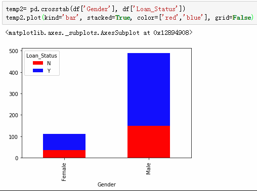
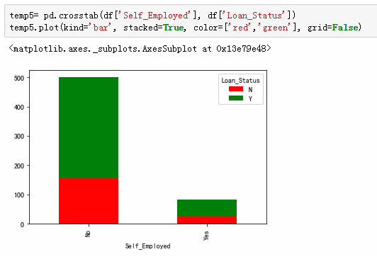
各属性与贷款批准与否的关系
我们用pandas.crosstab形成交叉表

绘制堆叠图
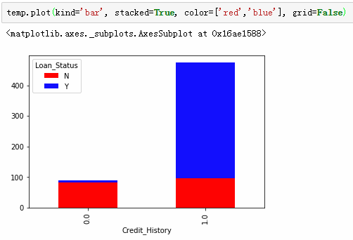
信用是一个有力的特征,信用好的更容易得到贷款。

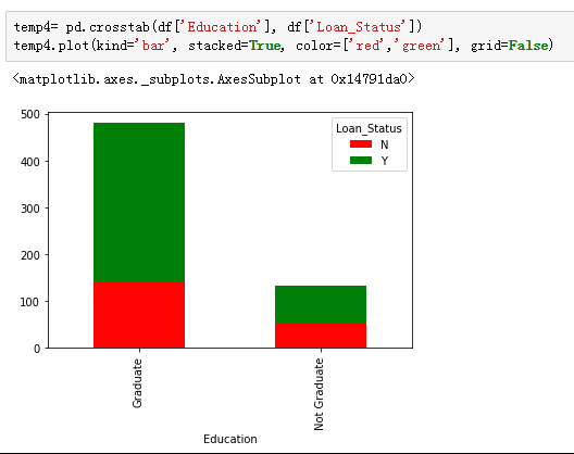
接受大学教育与否也是一个特征
a=df.groupby(['Credit_History','Gender','Loan_Status'])
dfa=pd.DataFrame(a.count()['Loan_ID'])
dfa

申请金额小更容易通过。
grid = sns.FacetGrid(df, col='Loan_Status', row='Dependents', size=2.2, aspect=2)
grid.map(plt.hist, 'LoanAmount', alpha=.5, bins=50)
grid.add_legend()

我们看不出家庭人数和借款额与Loan_Status的关系
我们可以从以上的图里发现一些关系和现实合理的假设:
1,有信用记录的人更容易得到贷款
2,受大学教育与否对是否贷款有些影响
3,结婚人士更容易得到贷款
4,申请金额小更容易通过
这四个特征将先用于初步训练模型
数据处理
数据处理通常是对空缺值,离群值和非数值变量进行处理。在处理时我们要衡量变量的缺失程度和特征的重要性,对一些具有意义的离群值要消除它的过度影响。
我们先对空缺值进行处理
该怎么处理空值呢?有以下几点:
1,大量样本缺失时,我们可能选择删除该变量,这类样本再加入模型可能影响模型结果。
2,适度样本缺失时,我们分两种情况:
a,连续型:做一个步长(step)。b,非连续型:把空值作为一类加入到变量中
3,缺失值不是很多,我们可以放入模型试试,也可以根据现有数据补全。
我们把训练集和测试集合并取出要预测的变量Loan_Status
train_df = pd.read_csv(r'C:\Users\Administrator\Desktop\train_u6lujuX_CVtuZ9i.csv',index_col=0)
test_df=pd.read_csv(r'C:\Users\Administrator\Desktop\test_Y3wMUE5_7gLdaTN.csv',index_col=0)#读取两个数据集合
把Loan_Status编码化(0,1),取出Loan_Status等于y待用
col_Loan_Status=pd.Categorical(train_df['Loan_Status'])
y=pd.DataFrame({'Loan_Status':col_Loan_Status.codes})
train_df=train_df.drop(['Loan_Status'],axis=1)
df=pd.concat((train_df,test_df),axis=0)
把两个收入相加生成新的列,看看他的分布
df['Income'] = df['ApplicantIncome'] + df['CoapplicantIncome']
df['Income'].hist(bins=50)

这是一个有偏分布,在做计算判断可能也会偏,我们可以让它平稳一点。
df['Income_log'] = np.log1p(df['Income'])
df.drop(['Income','ApplicantIncome','CoapplicantIncome'],axis=1,inplace=True)
df['Income_log'].hist(bins=25)
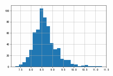
这样分布更符合正态分布
同样的我们也把LoanAmount进行对数处理,处理前先把空值填充,方法是从均值加减标准差随机取数
mean = df["LoanAmount"].mean()
std = df["LoanAmount"].std()
is_null = df["LoanAmount"].isnull().sum()
# compute random numbers between the mean, std and is_null
rand_LoanAmount = np.random.randint(mean - std, mean + std, size = is_null)
# fill NaN values in Age column with random values generated
LoanAmount_slice = df["LoanAmount"].copy()
LoanAmount_slice[np.isnan(LoanAmount_slice)] = rand_LoanAmount
df["LoanAmount"] = LoanAmount_slice
df["LoanAmount"] = df["LoanAmount"].astype(int)
对数处理
df['LoanAmount_log']=np.log1p(df['LoanAmount'])
df.drop(['LoanAmount'],axis=1,inplace=True)
看看还剩什么要处理
Married缺失值只有三个,我们使用pandas中fillna填充,先编码化
M={'Yes':1,'No':0}
df['Married']=df['Married'].map(M)
df['Married']=df['Married'].fillna(method='pad')
df['Married']=df['Married'].astype(int)
同样的方法对Gender,Self_Employed,Dependents,LoanAmount,Education

S={'Yes':1,'No':0}
df['Self_Employed']=df['Self_Employed'].map(S)
df['Self_Employed']=df['Self_Employed'].fillna(method='pad').astype(int)

df['Loan_Amount_Term']=df['Loan_Amount_Term'].fillna(method='pad').astype(int)

G={'Male':1,'Female':0}
df['Gender']=df['Gender'].map(G)
df['Gender']=df['Gender'].fillna(method='pad').astype(int)

df['Dependents'].replace(['0','1','2','3+'],[0,1,2,3],inplace=True)
df['Dependents']=df['Dependents'].fillna(method='pad').astype(int)

E={'Graduate':1,'Not Graduate':0}
df['Education']=df['Education'].map(E)
df['Education']=df['Education'].fillna(method='pad').astype(int)
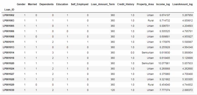
看看我们的数据。
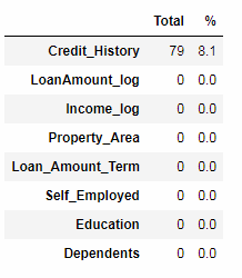
好多了,还剩下Property_Area和Credit_History的缺失值
对Property_Area的处理,由于数字是有大小的,如果对Property_Area数字编码的话可能数字的大小对模型产生影响,因此我们对它使用pandas自带的get_dummiesOne-Hot处理。实际上以上某些变量也可以用这个方法处理。
dummy_Property_Area=pd.get_dummies(df['Property_Area'])
df=pd.concat([df,dummy_Property_Area],axis=1)
df.drop(['Property_Area'],axis=1,inplace=True)
jiexialai对Credit_History进行处理
在这里我们可以对信用记录是否是缺失分为两类看看他们与是否批准贷款的分布
fig = plt.figure()
fig.set(alpha=0.2)
noCH=df.Loan_Status[pd.isnull(df.Credit_History)].value_counts()
CH = df.Loan_Status[pd.notnull(df.Credit_History)].value_counts()
df1=pd.DataFrame({'不缺失':CH,'缺失':noCH}).transpose()
df1.plot(kind='bar',stacked=True,color=['blue','red'])
plt.title("按信用记录是否缺失看是否贷款")
plt.xlabel("信用记录是否缺失")
plt.ylabel("人数")
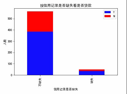

信用记录是缺失值的似乎更难得到贷款。
我把空值作为一类即,再对它One-Hot处理。
dummy_Credit_History=pd.get_dummies(df['Credit_History'])
df=pd.concat([df,dummy_Credit_History],axis=1)
df.drop(['Credit_History'],axis=1,inplace=True)
都处理完了。我们看看

特征建立
日平均还款的对数:用于衡量平均每日还款
df['Day_Payment']=cc['LoanAmount']/cc['Loan_Amount_Term']
df['Day_Payment'].fillna(df['Day_Payment'].mean(),inplace=True)
家庭收入比总收入和申报收入比总收入:用来衡量收入来源
aa = pd.read_csv(r'C:\Users\Administrator\Desktop\train_u6lujuX_CVtuZ9i.csv',index_col=0)
bb = pd.read_csv(r'C:\Users\Administrator\Desktop\test_Y3wMUE5_7gLdaTN.csv',index_col=0)#读取两个数据集合
cc=pd.concat((aa,bb),axis=0)
cc['ApplicantIncome']=np.log1p(cc['ApplicantIncome'])
cc['CoapplicantIncome']=np.log1p(cc['CoapplicantIncome'])
cc['Income']=cc['ApplicantIncome']+cc['CoapplicantIncome']
df['CoIncome_index']=cc['CoapplicantIncome']/cc['Income']
df['AppIncome_index']=cc['ApplicantIncome']/cc['Income']
建立机器学习模型
先把两个集合分开
D_train_df =df.loc[train_df.index]
D_test_df =df.loc[test_df.index]
D_train_df.shape,D_test_df.shape