逻辑回归中的梯度下降

这次使用了类的编程方法, 集成度、效率更高, 代码量更少, 使用更少的库

import numpy as np
import matplotlib.pyplot as plt


class LogisticRegression:
    def __init__(self,
                 learning_rate=0.001,
                 max_iter=100,
                 solver=None,
                 error=1e-5):  #设定模型参数
        print("------逻辑回归代码测试------")
        self.learning_rate = learning_rate
        self.max_iter = max_iter
        self.error = error
        solver_list = ['GD', 'newton-cg', 'lbfgs', 'sag', 'saga']  #其它求解方法后续会加入
        if solver == "GD" or solver == None:
            self.solver = "GD"
            print(
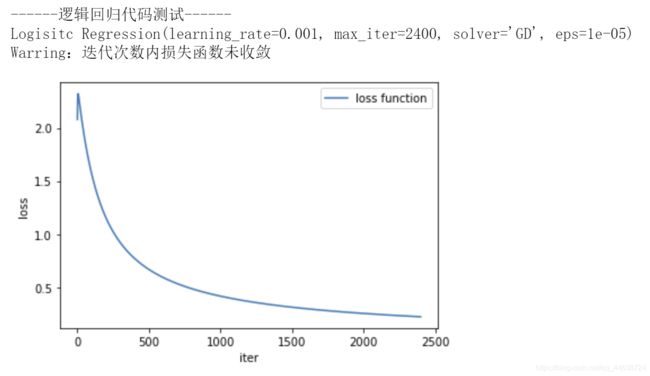
                "Logisitc Regression(learning_rate={0}, max_iter={1}, solver='{2}', eps={3})"
                .format(learning_rate, max_iter, solver, error))
        else:
            print(
                "Logistic Regression supports only solvers in ['GD', 'newton-cg', 'lbfgs', 'sag', 'saga'], got {0}"
                .format(solver))

    def pdf(self, x, mu, gamma, plot):  #绘制概率密度函数
        f = np.exp((mu - x) / gamma) / (gamma * (np.exp(
            (mu - x) / gamma) + 1)**2)
        if plot == True:
            plt.ylabel(f'$F(x)$')
            plt.xlabel(f"$x$")
            plt.vlines(mu, 0, max(f), linestyles="dashed")
            plt.title("PDF")
            plt.plot(x, f)
            plt.show()

    def cdf(self, x, mu, gamma, plot):  #绘制累计分布函数
        F = 1 / (1 + np.exp(-(x - mu) / gamma))
        if plot == True:
            plt.ylabel(f'$F(x)$')
            plt.xlabel(f"$x$")
            plt.vlines(0, 0, 1, linestyles="dashed")
            plt.title("CDF")
            plt.plot(x, F)
            plt.show()

    def fit(self, X, Y, beta=None, plot=None):  #训练模型
        x = np.array(X)
        y = np.array(Y)
        beta = np.zeros(x.shape[1])
        self.coef_ = beta
        n = len(y)
        Loss = [0]
        if self.solver == "GD":  #梯度下降法
            for i in range(self.max_iter):
                phi = 1 / (1 + np.exp(-np.dot(self.coef_, x.T)))
                self.coef_ = self.coef_ + self.learning_rate * np.dot(
                    (y.T - phi), x) / n
                Loss.append(-np.dot(y, np.log(phi).T))
                loss = abs(Loss[-1] - Loss[-2])
                if loss <= self.error:
                    break
                elif len(Loss) == self.max_iter and loss > self.error:
                    print('Warring：迭代次数内损失函数未收敛')
        if plot == True:
            plt.xlabel("iter")
            plt.ylabel("loss")
            plt.plot(Loss[1:-1])
            plt.legend(["loss function"])
            plt.show()
        if self.solver == "newton-cg":  #拟牛顿法
            print("拟牛顿法")

        if self.solver == "lbfgs":
            print("lbfgs")

    def predict_pro(self, testX):  #对新输入进行预测
        neg = 1 / (1 + np.exp(np.dot(self.coef_, testX.T)))[0]
        pos = 1 - neg
        return np.array([neg, pos])

用法

• 创建回归对象

LR = LogisticRegression(learning_rate=0.001, max_iter=2400, solver='GD')

• 给定输入输出

X = [[1, 20, 3], [1, 23, 7], [1, 31, 10], [1, 42, 13], [1, 50, 7], [1, 60, 5]]
Y = [0, 1, 1, 1, 0, 0]

• 训练模型

LR.fit(X,Y,plot=True) #可以用plot参数来控制是否绘制损失函数的收敛过程

• 结果
  
• 查看回归系数

LR.coef_

>>> array([-0.0015688 , -0.19926538,  0.91831361])

• 对新输入进行预测

testX=np.array([[1,28,8]])
LR.predict_pro(testX)

>>> array([0.14610166, 0.85389834])

对新输入样本的预测结果为: $P(Y=0|X)=0.14610166,P(Y=1|X)=1-P(Y=0|X)=0.85389834$

• 同时还可以查看逻辑斯蒂分布

data = np.arange(-30,30,0.01) #设定x
LR.cdf(data,2,4,True)
LR.pdf(data,2,4,True)

后面将陆续加入其它求解算法和惩罚项