
系统发育树是研究物种进化历史必不可少的信息,我们可以利用它得到一些重要历史线索,如:
- 生物多样性(物种形成或灭绝);
- 物种性状进化与多样化(Character evolution and diversification);
- 生物地理学(研究动植物的地理分布);
-
测试复杂进化模型;

Introduction to phylogenies in R
首先,安装系统发育分析所需的软件包
install CRAN Task View for phylogenetics to run, remove the comment character '#'
# install.packages("ctv")
# library("ctv")
# install.views("Phylogenetics")
# update.views("Phylogenetics")
# install.packages("ape")
# install.packages("geiger")
# install.packages("phytools")
# citation("geiger")
如何使用R进行系统发育树编辑
tree = "(((((((cow, pig),whale),(bat,(lemur,human))),(robin,iguana)),coelacanth),gold_fish),shark);"  # 从字符串中读取树文件
vert.tree <- read.tree(text=tree)
plot(vert.tree) # 普通可视化
plot(vert.tree,type="cladogram")
plot(unroot(vert.tree),type="unrooted")
plot(vert.tree,type="fan")
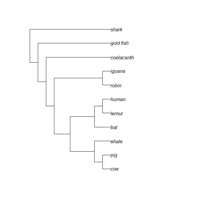


其实,此处的树文件就是一个字符串列表(列表还可以是数字型)。
> str(vert.tree)
List of 3
 $ edge     : int [1:20, 1:2] 12 13 14 15 16 17 18 18 17 16 ...
 $ Nnode    : int 10
 $ tip.label: chr [1:11] "cow" "pig" "whale" "bat" ...
 - attr(*, "class")= chr "phylo"
 - attr(*, "order")= chr "cladewise"
接下来,主要是看一下这些对象是如何存储在变量中的:
tree<-read.tree(text="(((A,B),(C,D)),E);")
plot(tree,type="cladogram",edge.width=2)
> tree$edge
     [,1] [,2]
[1,]    6    7
[2,]    7    8
[3,]    8    1
[4,]    8    2
[5,]    7    9
[6,]    9    3
[7,]    9    4
[8,]    6    5

> tree$tip.label
[1] "A" "B" "C" "D" "E"

> tree$Nnode
[1] 4

plot(tree,edge.width=2,label.offset=0.1,type="cladogram")
nodelabels()
tiplabels()
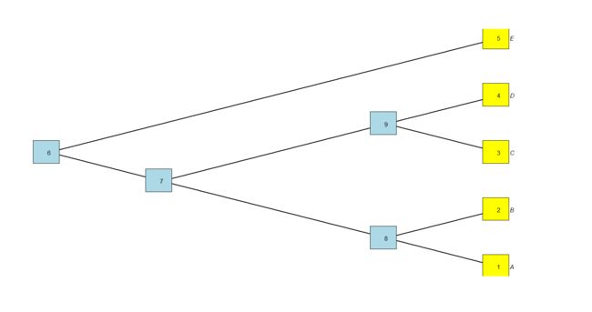
我们可以看到,树中所有分类单元之间的关系信息都包含在每条边的起始节点和结束节点中,共享共同起始节点编号的边是直接共同祖先的后代。
我们还可以测试树文件,编辑以及去除一些末端枝:

## (I'm going to first set the seed for repeatability)
set.seed(1)
## simulate a birth-death tree using phytools
tree<-pbtree(b=1,d=0.2,n=40)
## stopping criterion is 40 extant species, in this case
plotTree(tree)
nodelabels()
## ok, now extract the clade descended from node #62
tt62<-extract.clade(tree,62)
plotTree(tt62)

## now drop 10 tips from the tree (I'm going to pick them at random)
dtips<-sample(tree$tip.label,10)
dt<-drop.tip(tree,dtips)
plotTree(dt)

## we could also, say, drop all tips that go extinct before the present
## this is a fun way, but not the only way to do this:
plotTree(et<-drop.tip(tree,getExtinct(tree)),cex=0.7)

## rotating nodes
plotTree(tree,node.numbers=T)
## first, rotate about node #50
rt.50<-rotate(tree,50)
plotTree(rt.50)
## now rotate all nodes
rt.all<-rotateNodes(tree,"all")
plotTree(rt.all)
## ok, now let's re-root the tree at node #67
rr.67<-root(tree,node=67)
plotTree(rr.67)
## this creates a trifurcation at the root
## we could instead re-root at along an edge
rr.62<-reroot(tree,62,position=0.5*tree$edge.length[which(tree$edge[,2]==62)])
plotTree(rr.62)
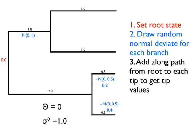
布朗模型(Brownian Motion)
布朗模型:
(1). 连续型性状进化的一个模型;
(2). 性状随着时间不断变化;
(3). 经过一段时间后,预期的状态将服从正态分布;
1. 什么是布朗运动?
(1). 有时称为维纳过程;
(2). 连续时间随机过程;
(3). 描述连续型性状的“随机演化”;
2. 布朗运动在何时才会发生?
(1). BM可以用来描述由大量独立的弱力组合而产生的运动;
(2). 加入许多小的自变量后,无论原始分布如何(中心极限定理),都会产生正态分布;

演化过程近似布朗运动
Ⅰ. 遗传漂变
Ⅱ. 随机改变
Ⅲ. 相对于考虑的时间间隔弱的自然选择
Ⅳ. 随时间随机变化的自然选择
3. 模拟布朗运动
- 模拟布朗运动需要从正态分布中提取值
- 分布的方差取决于σ2和t
- 沿着相邻分支的值从根添加到末端


系统发育独立差(Phylogenetic Independent Contrasts)
- PIC主要用来分析来自系统发育树的数据
- 检测性状之间进化相关性
- 我们可以将PIC看作是一种创建独立数据点的统计转换
系统发育独立差(Phylogenetic Independent Contrast, PIC)是去除性状分析中物种系统发育关系的一种方法,是美国进化生物学家 J. Felsenstein于1985年提出的。参考链接
当时,有动物学家检验了若干哺乳动物脑容量和体重的相关性。然而,所用统计方法都假设各个种的性状是相互独立的,采集自同一个正态分布的总体。由于不同种之间存在系统发育上的联系,因此不能直接套用常规统计模型,所以所得结果也就不可信了。在Felsenstein之前,一些学者已经意识到这个问题,但是都没能给出理想的解决方案。
Felsenstain认真思考了这个问题,并且认为:研究多个不同性状的相关性时,必须考虑系统发育关系。他提出:假设物种性状的进化服从布朗运动,那么用系统发育关系上最近的分类单元性状的差值,再经过枝长加权,就可以得到一组新的数据。这组新的数据去掉了进化信息的干扰,因此可以用常规统计方法检验。上述方法新获得的数据就称为系统发育独立差 (The Phylogenetic Independent Contrast, PIC)。
举例来说,如果要研究哺乳动物脑容量和体重的关系,就要先获得这些种之间的进化关系,也就是经过分子钟校订的进化树。然后再计算脑容量的PIC和体重的PIC,再用脑容量的PIC和体重的PIC建立线性模型,进行相关性检验。
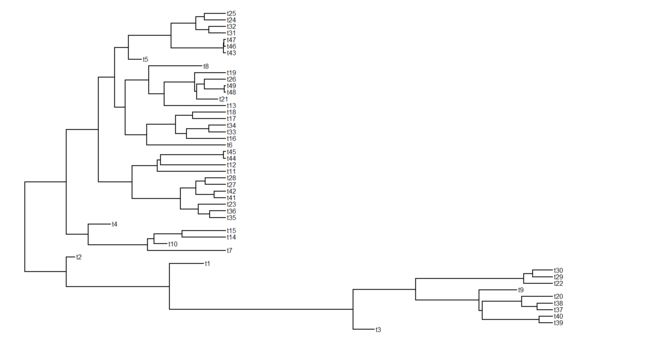
现在让我们来模拟一下布朗运动在树枝上的移动。坚持离散时间,我们首先需要一个离散时间的系统演化,我们可以用pbtree在phytools中进行模拟。
library(phytools)
t<-100 # total time
n<-30 # total taxa
b<-(log(n)-log(2))/t
tree<-pbtree(b=b,n=n,t=t,type="discrete")
## simulating with both taxa-stop (n) and time-stop (t) is
## performed via rejection sampling & may be slow
##
##   28 trees rejected before finding a tree
plotTree(tree)
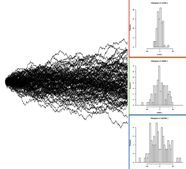
现在,为了在树的所有分支上进行模拟,我们只需要分别在每个分支上模拟,然后根据每个分支的父分支的结束状态“移动”每个子分支。我们可以这样做,记住,因为布朗演化的结果在每个时间步骤是独立于所有其他的时间步骤。
## simulate evolution along each edge
X<-lapply(tree$edge.length,function(x) c(0,cumsum(rnorm(n=x,sd=sqrt(sig2)))))
## reorder the edges of the tree for pre-order traversal
cw<-reorder(tree)
## now simulate on the tree
ll<-tree$edge.length+1
for(i in 1:nrow(cw$edge)){
    pp<-which(cw$edge[,2]==cw$edge[i,1])
    if(length(pp)>0) X[[i]]<-X[[i]]+X[[pp]][ll[pp]]
    else X[[i]]<-X[[i]]+X[[1]][1]
}
## get the starting and ending points of each edge for plotting
H<-nodeHeights(tree)
## plot the simulation
plot(H[1,1],X[[1]][1],ylim=range(X),xlim=range(H),xlab="time",ylab="phenotype")
for(i in 1:length(X)) lines(H[i,1]:H[i,2],X[[i]])
## add tip labels if desired
yy<-sapply(1:length(tree$tip.label),function(x,y) which(x==y),y=tree$edge[,2])
yy<-sapply(yy,function(x,y) y[[x]][length(y[[x]])],y=X)
text(x=max(H),y=yy,tree$tip.label)

## simulate Brownian evolution on a tree with fastBM
x<-fastBM(tree,sig2=sig2,internal=TRUE)
## visualize Brownian evolution on a tree
phenogram(tree,x,spread.labels=TRUE,spread.cost=c(1,0))
x<-sim.rates(tree,setNames(c(1,20),1:2),internal=TRUE)
phenogram(tree,x,colors=setNames(c("blue","red"),1:2),spread.labels=TRUE,spread.cost=c(1,0))

set.seed(100)
## transition matrix for the discrete trait simulation
Q<-matrix(c(-1,1,1,-1),2,2)
## simulated tree
tree<-pbtree(n=30,scale=1)
## simulate discrete character history
tree<-sim.history(tree,Q,anc="1")

## plot discrete character history on the tree
plotSimmap(tree,setNames(c("blue","red"),1:2),pts=F)

## simulate 5 taxon tree
tree<-pbtree(n=5,tip.label=LETTERS[1:5])
## 500 BM simulations
X<-fastBM(tree,nsim=500)
## plot tree
plot(rotateNodes(tree,"all"),edge.width=2,no.margin=TRUE)

## plot distribution across tips from 500 simulations
library(car)
scatterplotMatrix(t(X))

t <- 0:100  # time
sig2 <- 0.01
nsim <- 1000
## we'll simulate the steps from a uniform distribution
## with limits set to have the same variance (0.01) as before
X<-matrix(runif(n=nsim*(length(t)-1),min=-sqrt(3*sig2),max=sqrt(3*sig2)),nsim,length(t)-1)
X <- cbind(rep(0, nsim), t(apply(X, 1, cumsum)))
plot(t, X[1, ], xlab = "time", ylab = "phenotype", ylim = c(-2, 2), type = "l")
apply(X[2:nsim, ], 1, function(x, t) lines(t, x), t = t)

var(X[, length(t)])
hist(X[,length(t)])
plot(density(X[,length(t)]))

nsim=100
X <- matrix(rnorm(mean=0.02,n = nsim * (length(t) - 1), sd = sqrt(sig2/4)), nsim, length(t) - 1)
X <- cbind(rep(0, nsim), t(apply(X, 1, cumsum)))
plot(t, X[1, ], xlab = "time", ylab = "phenotype", ylim = c(-1, 3), type = "l")
apply(X[2:nsim, ], 1, function(x, t) lines(t, x), t = t)
在本教程中,我们将学习应用Felsenstein的独立对比方法来估计性状之间的进化相关性。Felsenstein发现一个以前已经认识到的问题,但这一问题没有得到充分的认识:即从统计分析的角度来看,物种数据不能被视为独立的数据点。
为了学习对比方法,我们首先需要学习一些用r语言拟合线性模型的基础知识。
## linear regression model is y = b0 + b*x + e
b0<-5.3
b<-0.75
x<-rnorm(n=100,sd=1)
y<-b0+b*x+rnorm(n=100,sd=0.2)
plot(x,y)
fit<-lm(y~x)
abline(fit)

> fit
Call: lm(formula = y ~ x)
Coefficients:
(Intercept)            x
     5.3123       0.7412
> summary(fit)

##
## Call:
## lm(formula = y ~ x)
##
## Residuals:
##      Min       1Q   Median       3Q      Max
## -0.52591 -0.12877 -0.01271  0.12295  0.57436
##
## Coefficients:
##             Estimate Std. Error t value Pr(>|t|)
## (Intercept)  5.33205    0.02129  250.39   <2e-16 ***
## x            0.73766    0.02103   35.08   <2e-16 ***
## ---
## Signif. codes:  0 '***' 0.001 '**' 0.01 '*' 0.05 '.' 0.1 ' ' 1
##
## Residual standard error: 0.2129 on 98 degrees of freedom
## Multiple R-squared:  0.9263, Adjusted R-squared:  0.9255
## F-statistic:  1231 on 1 and 98 DF,  p-value: < 2.2e-16

anova(fit)
## Analysis of Variance Table
##
## Response: y
##           Df Sum Sq Mean Sq F value    Pr(>F)
## x          1 55.804  55.804  1230.9 < 2.2e-16 ***
## Residuals 98  4.443   0.045
## ---
## Signif. codes:  0 '***' 0.001 '**' 0.01 '*' 0.05 '.' 0.1 ' ' 1

## coefficients of the fitted model
fit$coefficients
## (Intercept)           x
##   5.3320548   0.7376578

## p-value of the fitted model
anova(fit)[["Pr(>F)"]][1]
## [1] 2.758908e-57

foo<-function(){
    x<-rnorm(n=100)
    y<-rnorm(n=100)
    fit<-lm(y~x)
    setNames(c(fit$coefficients[2],anova(fit)[["Pr(>F)"]][1]),c("beta","p"))
}
X<-t(replicate(1000,foo()))
hist(X[,1],xlab="fitted beta",main="fitted beta")
hist(X[,2],xlab="p-value",main="p-value")

## expected value is the nominal type I error rate, 0.05
mean(X[,2]<=0.05)
## [1] 0.056

这个模拟非常简单地表明,当满足标准统计假设时,我们的参数估计是无偏的,并且第一类误差在标称水平或附近。
系统发育数据的困难在于,对于y的观测不再是独立的和相同的分布:
## load phytools
library(phytools)
## simulate a coalescent shaped tree
tree<-rcoal(n=100)
plotTree(tree,ftype="off")
## simulate uncorrelated Brownian evolution
x<-fastBM(tree)
y<-fastBM(tree)
par(mar=c(5.1,4.1,2.1,2.1))
plot(x,y)
fit<-lm(y~x)
abline(fit)

## this is a projection of the tree into morphospace
phylomorphospace(tree,cbind(x,y),label="off",node.size=c(0.5,0.7))
abline(fit)
从这个例子中我们可以看出,对于系统发育来说,诱发I类型的错误并不难。这是因为紧密相关的分类群具有高度相似的表型。换句话说,它们并不是关于树上x和y的演化过程的独立数据点.
PGLS系统发育广义最小二乘法
library(ape)
library(geiger)
library(nlme)
library(phytools)

anoleData <- read.csv("anolisDataAppended.csv", row.names = 1)
anoleTree <- read.tree("anolis.phy")
plot(anoleTree)
name.check(anoleTree, anoleData)

# Extract columns
host <- anoleData[, "hostility"]
awe <- anoleData[, "awesomeness"]

# Give them names
names(host) <- names(awe) <- rownames(anoleData)

# Calculate PICs
hPic <- pic(host, anoleTree)
aPic <- pic(awe, anoleTree)

# Make a model
picModel <- lm(hPic ~ aPic - 1)

# Yes, significant
summary(picModel)

##
## Call:
## lm(formula = hPic ~ aPic - 1)
##
## Residuals:
##    Min     1Q Median     3Q    Max
## -2.105 -0.419  0.010  0.314  4.999
##
## Coefficients:
##      Estimate Std. Error t value Pr(>|t|)
## aPic  -0.9776     0.0452   -21.6   <2e-16 ***
## ---
## Signif. codes:  0 '***' 0.001 '**' 0.01 '*' 0.05 '.' 0.1 ' ' 1
##
## Residual standard error: 0.897 on 98 degrees of freedom
## Multiple R-squared:  0.827,  Adjusted R-squared:  0.825
## F-statistic:  469 on 1 and 98 DF,  p-value: <2e-16

# plot results
plot(hPic ~ aPic)
abline(a = 0, b = coef(picModel))

# 我们可以直接使用PGLS
pglsModel <- gls(hostility ~ awesomeness, correlation = corBrownian(phy = anoleTree),
    data = anoleData, method = "ML")
summary(pglsModel)

## Generalized least squares fit by maximum likelihood
##   Model: hostility ~ awesomeness
##   Data: anoleData
##   AIC   BIC logLik
##   191 198.8 -92.49
##
## Correlation Structure: corBrownian
##  Formula: ~1
##  Parameter estimate(s):
## numeric(0)
##
## Coefficients:
##               Value Std.Error t-value p-value
## (Intercept)  0.1506   0.26263   0.573  0.5678
## awesomeness -0.9776   0.04516 -21.648  0.0000
##
##  Correlation:
##             (Intr)
## awesomeness -0.042
##
## Standardized residuals:
##      Min       Q1      Med       Q3      Max
## -0.76020 -0.39057 -0.04942  0.19597  1.07374
##
## Residual standard error: 0.8877
## Degrees of freedom: 100 total; 98 residual

coef(pglsModel)
## (Intercept) awesomeness
##      0.1506     -0.9776
plot(host ~ awe)
abline(a = coef(pglsModel)[1], b = coef(pglsModel)[2])
PGLS还可以使用多个预测变量:
pglsModel2 <- gls(hostility ~ ecomorph, correlation = corBrownian(phy = anoleTree),
    data = anoleData, method = "ML")
anova(pglsModel2)
## Denom. DF: 93
##             numDF F-value p-value
## (Intercept)     1 0.01847  0.8922
## ecomorph        6 0.21838  0.9700
coef(pglsModel2)
## (Intercept)  ecomorphGB   ecomorphT  ecomorphTC  ecomorphTG  ecomorphTW
##      0.4844     -0.6316     -1.0585     -0.8558     -0.4086     -0.4039

pglsModel3 <- gls(hostility ~ ecomorph * awesomeness, correlation = corBrownian(phy = anoleTree),
    data = anoleData, method = "ML")
anova(pglsModel3)
## Denom. DF: 86
##                      numDF F-value p-value
## (Intercept)              1     0.1  0.7280
## ecomorph                 6     1.4  0.2090
## awesomeness              1   472.9  <.0001
## ecomorph:awesomeness     6     3.9  0.0017

##还可以固定不同模型
# Does not converge - and this is difficult to fix!
pglsModelLambda <- gls(hostility ~ awesomeness, correlation = corPagel(1, phy = anoleTree,
    fixed = FALSE), data = anoleData, method = "ML")
# this is a problem with scale. We can do a quick fix by making the branch
# lengths longer. This will not affect the analysis other than rescaling a
# nuisance parameter
tempTree <- anoleTree
tempTree$edge.length <- tempTree$edge.length * 100
pglsModelLambda <- gls(hostility ~ awesomeness, correlation = corPagel(1, phy = tempTree,
    fixed = FALSE), data = anoleData, method = "ML")
summary(pglsModelLambda)
## Generalized least squares fit by maximum likelihood
##   Model: hostility ~ awesomeness
##   Data: anoleData
##     AIC   BIC logLik
##   72.56 82.98 -32.28
##
## Correlation Structure: corPagel
##  Formula: ~1
##  Parameter estimate(s):
##  lambda
## -0.1586
##
## Coefficients:
##               Value Std.Error t-value p-value
## (Intercept)  0.0612   0.01582   3.872   2e-04
## awesomeness -0.8777   0.03104 -28.273   0e+00
##
##  Correlation:
##             (Intr)
## awesomeness -1
##
## Standardized residuals:
##       Min        Q1       Med        Q3       Max
## -1.789463 -0.714775  0.003095  0.785093  2.232151
##
## Residual standard error: 0.371
## Degrees of freedom: 100 total; 98 residual

pglsModelOU <- gls(hostility ~ awesomeness, correlation = corMartins(1, phy = tempTree),
    data = anoleData, method = "ML")
summary(pglsModelOU)
## Generalized least squares fit by maximum likelihood
##   Model: hostility ~ awesomeness
##   Data: anoleData
##     AIC   BIC logLik
##   96.63 107.1 -44.32
##
## Correlation Structure: corMartins
##  Formula: ~1
##  Parameter estimate(s):
## alpha
## 4.442
##
## Coefficients:
##               Value Std.Error t-value p-value
## (Intercept)  0.1084   0.03953   2.743  0.0072
## awesomeness -0.8812   0.03658 -24.091  0.0000
##
##  Correlation:
##             (Intr)
## awesomeness -0.269
##
## Standardized residuals:
##     Min      Q1     Med      Q3     Max
## -1.8665 -0.8133 -0.1104  0.6475  2.0919
##
## Residual standard error: 0.3769
## Degrees of freedom: 100 total; 98 residual


系统发生信号
- Blomberg’s K statistic
- K >1系统发生信号很强
- K <1系统发生信号很弱
- Pagel’s lambda
- lambda =1 进化方向按照布朗模型
- lambda =0 进化方向没有相关性
library(geiger)
library(picante)
library(phytools)

anoleData <- read.csv("anolisDataAppended.csv", row.names = 1)
anoleTree <- read.tree("anolis.phy")
plot(anoleTree)
name.check(anoleTree, anoleData)

用体型大小来做两个主要的系统发育信号测试。第一个检验是Blomberg‘s K,它将PIC的方差与布朗运动模型下的方差进行比较。K=1表示亲属在BM下的相似程度,K<1表示在BM下存在较少的“系统发育信号”,而K>1表示存在更多的“系统发育信号”。从系统信号返回的显著p值告诉您存在显著的系统发育信号。也就是说,近亲比随机配对的物种更相似。
anoleSize <- anoleData[, 1]
names(anoleSize) <- rownames(anoleData)
phylosignal(anoleSize, anoleTree)
##       K PIC.variance.obs PIC.variance.rnd.mean PIC.variance.P
## 1 1.554           0.1389                 0.773          0.001
##   PIC.variance.Z
## 1         -3.913
phylosig(anoleTree, anoleSize, method = "K", test = T)
## $K
## [1] 1.554
##
## $P
## [1] 0.001
另一种检测系统发育信号的方法是Pagel的lambda。Lambda是一种相对于内部分支延伸尖端分支的树变换,使树越来越像一个完整的多段切除法。如果我们估计的λ=0,则推断这些性状没有系统发育信号。λ=1对应于布朗运动模型,0 不仅需要考虑数据类型,还要考虑适合数据的模型。不管是连续测量数据或离散数据,大多数都是遵循布朗运动模型(随着时间上下波动);或者是通过瞬间跳跃在状态之间(Brownian motion is a continuous-time stochastic process)。 推断祖先状态一直是系统发育比较生物学中一个重要的目标,本教程主要介绍如何在BM以及OU模型下重构祖先性状。第一个例子就是蜥蜴祖先体型大小的状态重建,这是一个连续型变量。 现在我们可以估计祖先的状态,还将计算方差&每个节点的95%置信区间: 然后,我们可以先根据布朗模型探讨连续特征的祖先状态重构的一些性质: 我们可以很容易地将这些估计与用于模拟数据的(正常unknown)生成值进行比较: 也可以使用布朗运动以外的其他角色进化模型来估计祖先的状态。例如,我们可以根据我们已经学到的OU模型来估计祖先的状态。需要注意的一点是:当选择参数(α)非常大时,祖先状态都会趋向于相同的值(拟合的最优,θ): 祖先状态估计当某些节点已知时。我们可以在祖先状态的MLE过程中从理论上确定任何内部节点的状态。在实践中,我们可以通过将长度为零的终端边缘附加到要修复的内部节点,然后将其作为分析中的另一个端值来处理。另一种可能也考虑到祖先状态不确定的可能性,即在内部节点上使用一个或多个状态上的信息先验概率密度,然后使用贝叶斯MCMC来估计祖先状态。让我们尝试一下,用一个非常糟糕的例子来估计祖先的特征,来自同一时期的尖端数据:有趋势的布朗进化。请注意,虽然理论上我们可以这样做,但我们并不适合这里的趋势模型。 接下来,重点介绍如何使用通常称为Mk模型的连续时间马尔可夫链模型来估计离散值性状的祖先特征状态。让我们从阿诺利树中提取数据,以便在这些分析中使用: $lik.anc变量主要包含临界祖先状态,也被称为“经验贝叶斯后验概率”: 以上概述的方法是使用MCMC从它们的后验概率分布中对性状历史进行采样,这叫做随机性状映射。模型是相同的,但在这种情况下,我们得到一个明确的历史样本,我们的离散型性状在树上的演变-而不是一个概率分布的性状在节点。例如,考虑到上面模拟的数据,我们可以生成如下的随机图: 单个随机字符映射并不意味着完全孤立-我们需要从随机映射的样本中查看整个分布。这可能有点令人难以抗拒。例如,以下代码从我们的数据集中生成100个随机字符映射,并在网格中绘制它们: 用一种更有意义的方式概括一组随机地图是可能的。例如,在我们的模型下,我们可以估计每种类型的变化数、在每种状态下花费的时间比例以及每个内部节点在每个状态下的后验概率。例如: 最后,由于我们在完全相同的模型下获得了这些推论,让我们将随机映射的后验概率与我们的边缘祖先状态进行比较。在前一种情况下,我们的概率是通过对祖先的联合(而不是边缘)概率分布的抽样来获得的。 这告诉我们,虽然联合和边缘祖先状态重建是不一样的,但联合随机抽样的边缘概率和边缘祖先状态是高度相关的-至少在这个案例研究中是这样的。 BAMM(Bayesian Analysis of Macroevolutionary Mixtures)是一个利用rjMCMC模型对物种形成、灭绝和性状进化的复杂动态进行建模的软件。然而,本教程将只集中于物种的形成和灭绝率的估计。运行BAMM需要两个主要输入文件:控制文件和系统发生树。 RPANDA利用最大似然分析,可以拟合不同的速率随时间变化的模型,并选择最优的拟合模型。RPANDA与BAMM主要有两个区别:# First let's look at what lambda does
anoleTreeLambda0 <- rescale(anoleTree, model = "lambda", 0)
anoleTreeLambda5 <- rescale(anoleTree, model = "lambda", 0.5)
par(mfcol = c(1, 3))
plot(anoleTree)
plot(anoleTreeLambda5)
plot(anoleTreeLambda0)
phylosig(anoleTree, anoleSize, method = "lambda", test = T)
## $lambda
## [1] 1.017
##
## $logL
## [1] -3.81
##
## $logL0
## [1] -60.02
##
## $P
## [1] 2.893e-26
lambdaModel <- fitContinuous(anoleTree, anoleSize, model = "lambda")
brownianModel <- fitContinuous(anoleTree, anoleSize)
nosigModel <- fitContinuous(anoleTreeLambda0, anoleSize)
lambdaModel$opt$aicc
## [1] 15.65
brownianModel$opt$aicc
## [1] 13.52
nosigModel$opt$aicc
## [1] 124.2
# Conclusion: Brownian model is best, no signal model is terrible
brownianModel <- fitContinuous(anoleTree, anoleSize)
OUModel <- fitContinuous(anoleTree, anoleSize, model = "OU")
EBModel <- fitContinuous(anoleTree, anoleSize, model = "EB")

# inspect results
brownianModel
## GEIGER-fitted comparative model of continuous data
##  fitted 'BM' model parameters:
##  sigsq = 0.136160
##  z0 = 4.065918
##
##  model summary:
##  log-likelihood = -4.700404
##  AIC = 13.400807
##  AICc = 13.524519
##  free parameters = 2
##
## Convergence diagnostics:
##  optimization iterations = 100
##  failed iterations = 0
##  frequency of best fit = 1.00
##
##  object summary:
##  'lik' -- likelihood function
##  'bnd' -- bounds for likelihood search
##  'res' -- optimization iteration summary
##  'opt' -- maximum likelihood parameter estimates
OUModel
## GEIGER-fitted comparative model of continuous data
##  fitted 'OU' model parameters:
##  alpha = 0.000000
##  sigsq = 0.136160
##  z0 = 4.065918
##
##  model summary:
##  log-likelihood = -4.700404
##  AIC = 15.400807
##  AICc = 15.650807
##  free parameters = 3
##
## Convergence diagnostics:
##  optimization iterations = 100
##  failed iterations = 0
##  frequency of best fit = 0.76
##
##  object summary:
##  'lik' -- likelihood function
##  'bnd' -- bounds for likelihood search
##  'res' -- optimization iteration summary
##  'opt' -- maximum likelihood parameter estimates
EBModel
## GEIGER-fitted comparative model of continuous data
##  fitted 'EB' model parameters:
##  a = -0.736271
##  sigsq = 0.233528
##  z0 = 4.066519
##
##  model summary:
##  log-likelihood = -4.285970
##  AIC = 14.571939
##  AICc = 14.821939
##  free parameters = 3
##
## Convergence diagnostics:
##  optimization iterations = 100
##  failed iterations = 0
##  frequency of best fit = 0.41
##
##  object summary:
##  'lik' -- likelihood function
##  'bnd' -- bounds for likelihood search
##  'res' -- optimization iteration summary
##  'opt' -- maximum likelihood parameter estimates

# calculate AIC weights
bmAICC <- brownianModel$opt$aicc
ouAICC <- OUModel$opt$aicc
ebAICC <- EBModel$opt$aicc

aicc <- c(bmAICC, ouAICC, ebAICC)
aiccD <- aicc - min(aicc)
aw <- exp(-0.5 * aiccD)
aiccW <- aw/sum(aw)
aiccW
## [1] 0.5353 0.1849 0.2798
It is important to realize that measurement error can bias your inferences with fitting these models towards OU. Fortunately, we can easily account for that in fitContinuous.


# We measured 20 anoles per species, and the standard deviation within each
# species was, on average, 0.05
seSize <- 0.05/sqrt(20)

# redo with measurement error
brownianModel <- fitContinuous(anoleTree, anoleSize, SE = seSize)
OUModel <- fitContinuous(anoleTree, anoleSize, model = "OU", SE = seSize)
EBModel <- fitContinuous(anoleTree, anoleSize, model = "EB", SE = seSize)


# calculate AIC weights
bmAICC <- brownianModel$opt$aicc
ouAICC <- OUModel$opt$aicc
ebAICC <- EBModel$opt$aicc

aicc <- c(bmAICC, ouAICC, ebAICC)
aiccD <- aicc - min(aicc)
aw <- exp(-0.5 * aiccD)
aiccW <- aw/sum(aw)
aiccW
## [1] 0.5346 0.1846 0.2808
重构祖先状态

## load libraries
library(phytools)
## read tree from file
tree<-read.tree("anole.tre") ## or
tree<-read.tree("http://www.phytools.org/Ilhabela2015/data/anole.tre")
## plot tree
plotTree(tree,type="fan",ftype="i")
## setEnv=TRUE for this type is experimental. please be patient with bugs

## read data
svl<-read.csv("svl.csv",row.names=1) ## or
svl<-read.csv("http://www.phytools.org/Ilhabela2015/data/svl.csv",
    row.names=1)
## change this into a vector
svl<-as.matrix(svl)[,1]
svl
##            ahli         alayoni         alfaroi        aliniger
##        4.039125        3.815705        3.526655        4.036557
##        allisoni         allogus   altitudinalis         alumina
##        4.375390        4.040138        3.842994        3.588941
##       alutaceus     angusticeps     argenteolus     argillaceus
##        3.554891        3.788595        3.971307        3.757869
##         armouri   bahorucoensis        baleatus        baracoae
##        4.121684        3.827445        5.053056        5.042780
##       barahonae        barbatus        barbouri        bartschi
##        5.076958        5.003946        3.663932        4.280547
##         bremeri        breslini    brevirostris        caudalis
##        4.113371        4.051111        3.874155        3.911743
##       centralis  chamaeleonides    chlorocyanus     christophei
##        3.697941        5.042349        4.275448        3.884652
##       clivicola     coelestinus        confusus           cooki
##        3.758726        4.297965        3.938442        4.091535
##    cristatellus    cupeyalensis         cuvieri    cyanopleurus
##        4.189820        3.462014        4.875012        3.630161
##         cybotes     darlingtoni       distichus dolichocephalus
##        4.210982        4.302036        3.928796        3.908550
##       equestris      etheridgei   eugenegrahami       evermanni
##        5.113994        3.657991        4.128504        4.165605
##         fowleri         garmani         grahami           guafe
##        4.288780        4.769473        4.154274        3.877457
##       guamuhaya         guazuma       gundlachi       haetianus
##        5.036953        3.763884        4.188105        4.316542
##      hendersoni      homolechis           imias    inexpectatus
##        3.859835        4.032806        4.099687        3.537439
##       insolitus        isolepis           jubar           krugi
##        3.800471        3.657088        3.952605        3.886500
##      lineatopus   longitibialis        loysiana          lucius
##        4.128612        4.242103        3.701240        4.198915
##    luteogularis      macilentus        marcanoi          marron
##        5.101085        3.715765        4.079485        3.831810
##         mestrei       monticola          noblei        occultus
##        3.987147        3.770613        5.083473        3.663049
##         olssoni        opalinus      ophiolepis        oporinus
##        3.793899        3.838376        3.637962        3.845670
##        paternus        placidus       poncensis        porcatus
##        3.802961        3.773967        3.820378        4.258991
##          porcus      pulchellus         pumilis quadriocellifer
##        5.038034        3.799022        3.466860        3.901619
##      reconditus        ricordii     rubribarbus          sagrei
##        4.482607        5.013963        4.078469        4.067162
##    semilineatus        sheplani         shrevei      singularis
##        3.696631        3.682924        3.983003        4.057997
##      smallwoodi         strahmi       stratulus     valencienni
##        5.035096        4.274271        3.869881        4.321524
##       vanidicus    vermiculatus        websteri       whitemani
##        3.626206        4.802849        3.916546        4.097479
fit<-fastAnc(tree,svl,vars=TRUE,CI=TRUE)
fit

## $ace
##      101      102      103      104      105      106      107      108
## 4.065918 4.045601 4.047993 4.066923 4.036743 4.049514 4.054528 4.045218
##      109      110      111      112      113      114      115      116
## 3.979493 3.952440 3.926814 3.964414 3.995835 3.948034 3.955203 3.977842
##      117      118      119      120      121      122      123      124
## 4.213995 4.240867 4.248450 4.257574 4.239061 4.004120 4.007024 4.015249
##      125      126      127      128      129      130      131      132
## 4.006720 3.992617 3.925848 3.995759 4.049619 3.930793 3.908343 3.901518
##      133      134      135      136      137      138      139      140
## 3.885086 4.040356 4.060970 3.987789 3.951878 3.814014 3.707733 3.926147
##      141      142      143      144      145      146      147      148
## 3.988745 4.167983 4.157021 4.166146 4.146362 4.146132 4.159052 4.113267
##      149      150      151      152      153      154      155      156
## 4.133069 4.222223 4.461376 4.488496 4.437250 4.512071 4.953146 5.033253
##      157      158      159      160      161      162      163      164
## 4.962377 5.009025 5.018389 3.974900 3.880482 3.859268 3.859265 3.871895
##      165      166      167      168      169      170      171      172
## 3.899914 3.807943 3.826619 4.151598 3.760446 3.654324 3.676713 3.825559
##      173      174      175      176      177      178      179      180
## 3.747726 3.813974 3.803077 3.702349 3.566476 3.678236 3.675620 3.662452
##      181      182      183      184      185      186      187      188
## 3.563181 3.645426 4.017460 4.113689 4.229393 4.381609 4.243153 5.041281
##      189      190      191      192      193      194      195      196
## 5.051563 5.051719 5.057591 4.183653 4.151505 4.113279 3.969795 3.905122
##      197      198      199
## 4.191810 4.161419 4.092141
##
## $var
##         101         102         103         104         105         106
## 0.011775189 0.008409641 0.009452076 0.011870028 0.014459672 0.018112713
##         107         108         109         110         111         112
## 0.011685860 0.007268889 0.014487712 0.012814461 0.010852276 0.010048935
##         113         114         115         116         117         118
## 0.006240382 0.009816255 0.008377720 0.006250414 0.015406961 0.015306088
##         119         120         121         122         123         124
## 0.008914737 0.008485896 0.016998370 0.014850114 0.012880197 0.011964472
##         125         126         127         128         129         130
## 0.010525923 0.010528040 0.013248168 0.012789504 0.013568841 0.013971730
##         131         132         133         134         135         136
## 0.010048937 0.009535820 0.008387455 0.008359158 0.010126605 0.012608132
##         137         138         139         140         141         142
## 0.013951936 0.018502968 0.014105896 0.018182598 0.017745869 0.012861889
##         143         144         145         146         147         148
## 0.014828558 0.011891297 0.008732027 0.008604618 0.010009986 0.007660375
##         149         150         151         152         153         154
## 0.006817879 0.012378867 0.015540878 0.014154484 0.012761730 0.011952420
##         155         156         157         158         159         160
## 0.005064274 0.002463170 0.006924118 0.003953467 0.003509809 0.011102798
##         161         162         163         164         165         166
## 0.011378573 0.011045003 0.011682628 0.011560333 0.012242267 0.011462597
##         167         168         169         170         171         172
## 0.008888509 0.014206315 0.014405121 0.006290501 0.005434707 0.014714164
##         173         174         175         176         177         178
## 0.010884130 0.014842361 0.011333759 0.012932194 0.007449222 0.011094079
##         179         180         181         182         183         184
## 0.011015666 0.012850744 0.005326252 0.012876076 0.021615405 0.014608411
##         185         186         187         188         189         190
## 0.013155037 0.021043877 0.012658226 0.004540141 0.003540634 0.002698421
##         191         192         193         194         195         196
## 0.001277775 0.011837709 0.012449062 0.013536624 0.015848988 0.008788712
##         197         198         199
## 0.015789566 0.013529210 0.009534335
##
## $CI95
##         [,1]     [,2]
## 101 3.853231 4.278604
## 102 3.865861 4.225341
## 103 3.857439 4.238548
## 104 3.853382 4.280465
## 105 3.801056 4.272430
## 106 3.785731 4.313298
## 107 3.842649 4.266406
## 108 3.878112 4.212323
## 109 3.743577 4.215408
## 110 3.730566 4.174314
## 111 3.722632 4.130995
## 112 3.767935 4.160893
## 113 3.841003 4.150668
## 114 3.753844 4.142225
## 115 3.775804 4.134601
## 116 3.822885 4.132799
## 117 3.970710 4.457279
## 118 3.998380 4.483354
## 119 4.063391 4.433509
## 120 4.077021 4.438127
## 121 3.983520 4.494601
## 122 3.765272 4.242968
## 123 3.784582 4.229467
## 124 3.800860 4.229639
## 125 3.805632 4.207808
## 126 3.791509 4.193725
## 127 3.700250 4.151445
## 128 3.774102 4.217417
## 129 3.821307 4.277930
## 130 3.699117 4.162469
## 131 3.711864 4.104822
## 132 3.710121 4.092915
## 133 3.705584 4.064589
## 134 3.861156 4.219555
## 135 3.863733 4.258207
## 136 3.767708 4.207869
## 137 3.720366 4.183390
## 138 3.547403 4.080624
## 139 3.474947 3.940519
## 140 3.661855 4.190439
## 141 3.727646 4.249843
## 142 3.945699 4.390267
## 143 3.918347 4.395695
## 144 3.952414 4.379879
## 145 3.963210 4.329515
## 146 3.964320 4.327943
## 147 3.962955 4.355150
## 148 3.941721 4.284813
## 149 3.971230 4.294907
## 150 4.004152 4.440293
## 151 4.217036 4.705715
## 152 4.255309 4.721682
## 153 4.215833 4.658667
## 154 4.297789 4.726352
## 155 4.813665 5.092627
## 156 4.935977 5.130528
## 157 4.799283 5.125471
## 158 4.885787 5.132263
## 159 4.902272 5.134507
## 160 3.768375 4.181425
## 161 3.671408 4.089556
## 162 3.653282 4.065255
## 163 3.647416 4.071113
## 164 3.661158 4.082632
## 165 3.683050 4.116777
## 166 3.598098 4.017787
## 167 3.641833 4.011406
## 168 3.917985 4.385211
## 169 3.525204 3.995688
## 170 3.498871 3.809777
## 171 3.532221 3.821205
## 172 3.587807 4.063310
## 173 3.543245 3.952207
## 174 3.575189 4.052760
## 175 3.594415 4.011738
## 176 3.479458 3.925240
## 177 3.397311 3.735642
## 178 3.471792 3.884680
## 179 3.469907 3.881332
## 180 3.440264 3.884639
## 181 3.420138 3.706225
## 182 3.423020 3.867833
## 183 3.729297 4.305622
## 184 3.876793 4.350585
## 185 4.004590 4.454196
## 186 4.097282 4.665937
## 187 4.022636 4.463670
## 188 4.909215 5.173347
## 189 4.934937 5.168189
## 190 4.949904 5.153533
## 191 4.987529 5.127654
## 192 3.970403 4.396903
## 193 3.932817 4.370192
## 194 3.885239 4.341319
## 195 3.723046 4.216545
## 196 3.721376 4.088869
## 197 3.945523 4.438096
## 198 3.933441 4.389397
## 199 3.900759 4.283523

## as we discussed in class, 95% CIs can be broad
fit$CI[1,]
## [1] 3.853231 4.278604

range(svl)
## [1] 3.462014 5.113994

## projection of the reconstruction onto the edges of the tree
obj<-contMap(tree,svl,plot=FALSE)
plot(obj,type="fan",legend=0.7*max(nodeHeights(tree)))

## projection of the tree into phenotype space
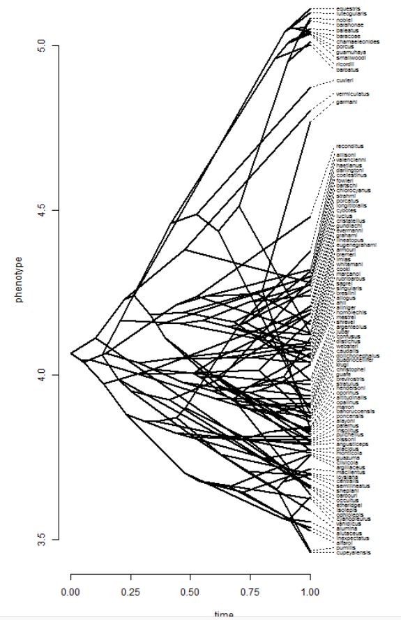
phenogram(tree,svl,fsize=0.6,spread.costs=c(1,0))
## Optimizing the positions of the tip labels...
## simulate a tree & some data
tree<-pbtree(n=26,scale=1,tip.label=LETTERS[26:1])
## simulate with ancestral states
x<-fastBM(tree,internal=TRUE)
## ancestral states
a<-x[as.character(1:tree$Nnode+Ntip(tree))]
## tip data
x<-x[tree$tip.label]

fit<-fastAnc(tree,x,CI=TRUE)
fit

## $ace
##          27          28          29          30          31          32
## -0.01383743 -0.43466511 -0.78496842 -0.92652372 -0.97992735 -1.06606765
##          33          34          35          36          37          38
## -1.19242145 -0.77435425 -1.33427168 -0.77148395  0.37519774  0.35486511
##          39          40          41          42          43          44
##  0.78011325  0.63488391  1.19427496 -0.20165383 -0.17792873  1.07419593
##          45          46          47          48          49          50
##  1.45924828  1.55175294  1.75289132  2.16445039  1.81192553  0.68319366
##          51
##  0.81241807
##
## $CI95
##          [,1]       [,2]
## 27 -0.8879801  0.8603052
## 28 -1.2581222  0.3887920
## 29 -1.4652988 -0.1046380
## 30 -1.5538351 -0.2992123
## 31 -1.4449545 -0.5149002
## 32 -1.4966267 -0.6355086
## 33 -1.4920621 -0.8927808
## 34 -1.1230122 -0.4256963
## 35 -1.4863921 -1.1821513
## 36 -1.2746445 -0.2683234
## 37 -0.3797317  1.1301272
## 38 -0.4031915  1.1129217
## 39  0.1541249  1.4061016
## 40  0.5162435  0.7535243
## 41  1.0781703  1.3103796
## 42 -0.7364614  0.3331537
## 43 -0.6011442  0.2452867
## 44  0.4157610  1.7326308
## 45  0.8942088  2.0242878
## 46  0.9951790  2.1083269
## 47  1.2382347  2.2675479
## 48  1.9117253  2.4171755
## 49  1.3260228  2.2978283
## 50  0.3463241  1.0200632
## 51  0.5937687  1.0310674
plot(a,fit$ace,xlab="true states",ylab="estimated states")
lines(range(c(x,a)),range(c(x,a)),lty="dashed",col="red") ## 1:1 line

##
对祖先状态估计最常见的批评之一是,围绕祖先状态的不确定性可能很大;而且,这种不确定性常常被忽略。让我们通过在祖先值上获得95%的CI来解决这一问题,然后让我们表明,95%的CI在大约95%的时间内包含生成值:
##
## first, let's go back to our previous dataset
print(fit)
mean(((a>=fit$CI95[,1]) + (a<=fit$CI95[,2]))==2)
## [1] 0.92

## custom function that conducts a simulation, estimates ancestral
## states, & returns the fraction on 95% CI
foo<-function(){
    tree<-pbtree(n=100)
    x<-fastBM(tree,internal=TRUE)
    fit<-fastAnc(tree,x[1:length(tree$tip.label)],CI=TRUE)
    mean(((x[1:tree$Nnode+length(tree$tip.label)]>=fit$CI95[,1]) +
        (x[1:tree$Nnode+length(tree$tip.label)]<=fit$CI95[,2]))==2)
}
## conduct 100 simulations
pp<-replicate(100,foo())
mean(pp)

## [1] 0.9448485

这表明,虽然CI可以很大,但当模型正确时,它们将包括生成值(1-α)%的时间
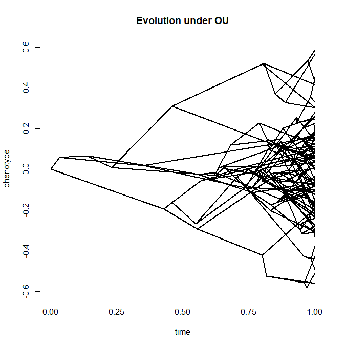
## simulate tree & data under the OU model
alpha<-2
tree<-pbtree(n=100,scale=1)
x<-fastBM(tree,internal=TRUE,model="OU",alpha=alpha,sig2=0.2)
## Warning: alpha but not theta specified in OU model, setting theta to a.
a<-x[as.character(1:tree$Nnode+Ntip(tree))]
x<-x[tree$tip.label]
phenogram(tree,c(x,a),ftype="off",spread.labels=FALSE)
title("Evolution under OU")
## fit the model (this may be slow)
fit<-anc.ML(tree,x,model="OU")
fit

## $sig2
## [1] 0.05573428
##
## $alpha
## [1] 1e-08
##
## $ace
##           101           102           103           104           105
##  9.963462e-03  2.244757e-02  2.240573e-02 -5.931035e-02 -4.329498e-02
##           106           107           108           109           110
## -3.480964e-02 -4.081294e-02 -1.143122e-01 -2.263273e-02  4.155330e-02
##           111           112           113           114           115
##  4.264017e-02 -1.810736e-02 -9.407912e-02 -1.363360e-01 -6.611306e-02
##           116           117           118           119           120
## -1.392603e-02 -3.488464e-02 -9.974915e-02 -1.471439e-01 -1.667432e-01
##           121           122           123           124           125
## -1.680456e-01  2.899822e-02  4.833528e-02  3.506143e-02  1.868645e-02
##           126           127           128           129           130
##  4.748435e-02  3.448893e-02  3.250233e-02 -1.538064e-03  5.460770e-02
##           131           132           133           134           135
##  1.287799e-01  1.331156e-01  1.469378e-01  8.486024e-03  6.439102e-03
##           136           137           138           139           140
## -5.997895e-02 -2.624823e-02  1.156061e-01  1.450449e-01  1.643474e-01
##           141           142           143           144           145
##  8.871516e-02 -1.500705e-01 -2.088446e-01 -1.485247e-01 -9.546454e-02
##           146           147           148           149           150
## -1.648921e-01 -1.003483e-01 -1.122847e-01 -9.953868e-02  2.319007e-01
##           151           152           153           154           155
##  4.114431e-02  3.261996e-02  5.558858e-02 -1.093121e-03 -2.343046e-03
##           156           157           158           159           160
## -9.063816e-05 -3.395186e-02 -7.084372e-02 -2.180441e-03 -9.891307e-02
##           161           162           163           164           165
## -3.951237e-02 -3.874053e-02 -2.391682e-02  9.737577e-02 -3.801571e-02
##           166           167           168           169           170
## -3.578902e-02 -2.162303e-02 -5.260689e-03 -1.308687e-02 -2.051804e-02
##           171           172           173           174           175
##  1.033658e-02  2.185436e-03  4.877736e-02  9.016846e-02 -6.244681e-03
##           176           177           178           179           180
##  2.600085e-03 -2.081362e-02 -6.850276e-02 -1.012200e-01 -9.815220e-02
##           181           182           183           184           185
## -9.432228e-02 -9.482774e-02 -1.266490e-01 -3.097925e-01 -1.008618e-01
##           186           187           188           189           190
## -1.202127e-02 -1.335903e-02 -3.088787e-04 -1.270292e-01  7.848848e-03
##           191           192           193           194           195
##  2.054886e-01  2.441548e-01 -4.855077e-02 -1.614209e-02 -3.053233e-02
##           196           197           198           199
## -5.844232e-02  2.570525e-02  2.987429e-02 -1.579888e-01
##
## $logLik
## [1] 263.5128
##
## $counts
## function gradient
##        8        8
##
## $convergence

## [1] 0
##
## $message
## [1] "CONVERGENCE: REL_REDUCTION_OF_F <= FACTR*EPSMCH"
##
## $model
## [1] "OU"
##
## attr(,"class")
## [1] "anc.ML"

plot(a,fit$ace,xlab="true values",ylab="estimated under OU")
lines(range(x),range(x),lty="dashed",col="red")
title("ancestral states estimated under OU")

tree<-pbtree(n=100,scale=1)
## simulate data with a trend
x<-fastBM(tree,internal=TRUE,mu=3)
phenogram(tree,x,ftype="off",spread.labels=FALSE)

a<-x[as.character(1:tree$Nnode+Ntip(tree))]
x<-x[tree$tip.label]
## let's see how bad we do if we ignore the trend
plot(a,fastAnc(tree,x),xlab="true values",
    ylab="estimated states under BM")
lines(range(c(x,a)),range(c(x,a)),lty="dashed",col="red")
title("estimated without prior information")


## incorporate prior knowledge
pm<-setNames(c(1000,rep(0,tree$Nnode)),
    c("sig2",1:tree$Nnode+length(tree$tip.label)))
## the root & two randomly chosen nodes
nn<-as.character(c(length(tree$tip.label)+1,
    sample(2:tree$Nnode+length(tree$tip.label),2)))
pm[nn]<-a[as.character(nn)]
## prior variance
pv<-setNames(c(1000^2,rep(1000,length(pm)-1)),names(pm))
pv[as.character(nn)]<-1e-100
## run MCMC
mcmc<-anc.Bayes(tree,x,ngen=100000,
    control=list(pr.mean=pm,pr.var=pv,
    a=pm[as.character(length(tree$tip.label)+1)],
    y=pm[as.character(2:tree$Nnode+length(tree$tip.label))]))

anc.est<-colMeans(mcmc[201:1001,
    as.character(1:tree$Nnode+length(tree$tip.label))])
plot(a[names(anc.est)],anc.est,xlab="true values",
    ylab="estimated states using informative prior")
lines(range(c(x,a)),range(c(x,a)),lty="dashed",col="red")
title("estimated using informative prior")


require(phytools)
data(anoletree)
## this is just to pull out the tip states from the
## data object - normally we would read this from file
x<-getStates(anoletree,"tips")
tree<-anoletree
rm(anoletree)
tree

##
## Phylogenetic tree with 82 tips and 81 internal nodes.
##
## Tip labels:
##  Anolis_ahli, Anolis_allogus, Anolis_rubribarbus, Anolis_imias, Anolis_sagrei, Anolis_bremeri, ...
##
## Rooted; includes branch lengths.
plotTree(tree,type="fan",fsize=0.8,ftype="i")

## estimate ancestral states under a ER model
fitER<-ace(x,tree,model="ER",type="discrete")
fitER

##
##     Ancestral Character Estimation
##
## Call: ace(x = x, phy = tree, type = "discrete", model = "ER")
##
##     Log-likelihood: -78.04604
##
## Rate index matrix:
##    CG GB TC TG Tr Tw
## CG  .  1  1  1  1  1
## GB  1  .  1  1  1  1
## TC  1  1  .  1  1  1
## TG  1  1  1  .  1  1
## Tr  1  1  1  1  .  1
## Tw  1  1  1  1  1  .
##
## Parameter estimates:
##  rate index estimate std-err
##           1   0.0231   0.004
##
## Scaled likelihoods at the root (type '...$lik.anc' to get them for all nodes):
##          CG          GB          TC          TG          Tr          Tw
## 0.018197565 0.202238628 0.042841575 0.428609607 0.004383532 0.303729093

round(fitER$lik.anc,3)
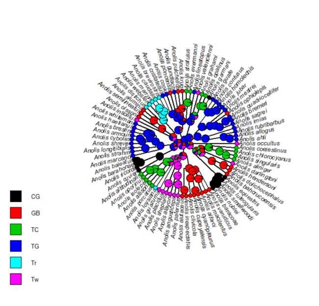
plotTree(tree,type="fan",fsize=0.8,ftype="i")
nodelabels(node=1:tree$Nnode+Ntip(tree),
    pie=fitER$lik.anc,piecol=cols,cex=0.5)
tiplabels(pie=to.matrix(x,sort(unique(x))),piecol=cols,cex=0.3)
add.simmap.legend(colors=cols,prompt=FALSE,x=0.9*par()$usr[1],
    y=-max(nodeHeights(tree)),fsize=0.8)
## simulate single stochastic character map using empirical Bayes method
mtree<-make.simmap(tree,x,model="ER")
plotSimmap(mtree,cols,type="fan",fsize=0.8,ftype="i")
add.simmap.legend(colors=cols,prompt=FALSE,x=0.9*par()$usr[1],
    y=-max(nodeHeights(tree)),fsize=0.8)

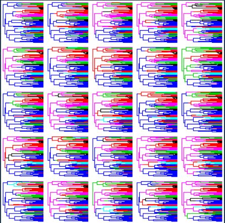
mtrees<-make.simmap(tree,x,model="ER",nsim=100)
par(mfrow=c(10,10))
null<-sapply(mtrees,plotSimmap,colors=cols,lwd=1,ftype="off")
pd<-describe.simmap(mtrees,plot=FALSE)
pd
plot(pd,fsize=0.6,ftype="i")

## now let's plot a random map, and overlay the posterior probabilities
plotSimmap(mtrees[[1]],cols,type="fan",fsize=0.8,ftype="i")
nodelabels(pie=pd$ace,piecol=cols,cex=0.5)
add.simmap.legend(colors=cols,prompt=FALSE,x=0.9*par()$usr[1],
    y=-max(nodeHeights(tree)),fsize=0.8)

plot(fitER$lik.anc,pd$ace,xlab="marginal ancestral states",
    ylab="posterior probabilities from stochastic mapping")
lines(c(0,1),c(0,1),lty="dashed",col="red",lwd=2)

实操演练
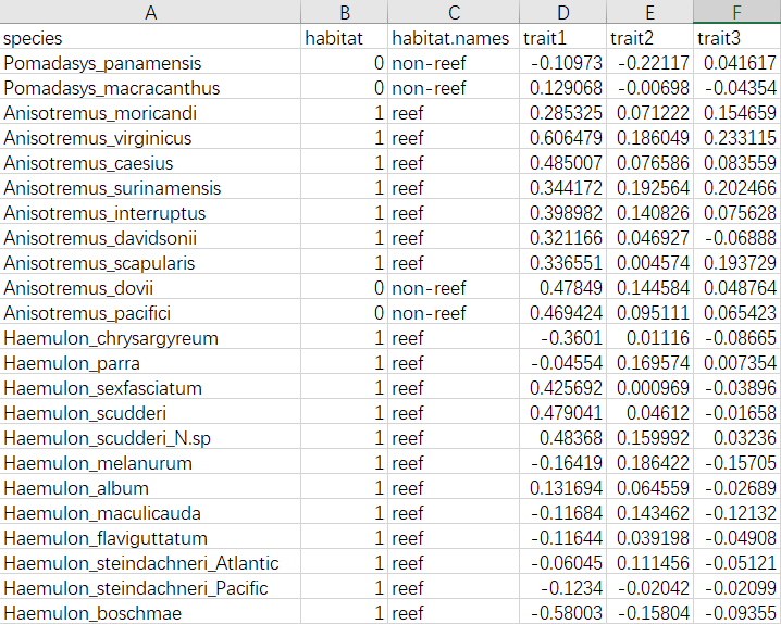
library(geiger)
gruntTree <- read.tree("grunts.phy")
gruntData <- read.csv("grunts.csv", row.names=1)
name.check(gruntTree, gruntData)

library(nlme)
plot(trait2~trait1, data=gruntData)
###run PGLS
pglsResult<-gls(trait1~trait2, cor=corBrownian(phy=gruntTree), data=gruntData, method="ML")
pglsResultOU<-gls(trait1~trait2, cor=corMartins(1, phy=gruntTree, fixed=F), data=gruntData, method="ML")
pglsResultPagel<-gls(trait1~trait2, cor=corPagel(1, phy=gruntTree, fixed=F), data=gruntData, method="ML")
anova(pglsResult, pglsResultOU, pglsResultPagel)

##                 Model df      AIC      BIC     logLik   Test  L.Ratio
## pglsResult          1  3 59.81018 65.54625 -26.905088
## pglsResultOU        2  4 30.42696 38.07506 -11.213482 1 vs 2 31.38321
## pglsResultPagel     3  4 22.83320 30.48129  -7.416599
##                 p-value
## pglsResult
## pglsResultOU     <.0001
## pglsResultPagel

# the main one is the lowest AIC, choose that
anova(pglsResultPagel)

## Denom. DF: 48
##             numDF  F-value p-value
## (Intercept)     1 0.004714  0.9455
## trait2          1 6.053490  0.0175

# yes there is a relationship.
results<-matrix(nrow=3, ncol=3)

for(i in 3:5) {
  xx <- gruntData[,i]
  names(xx) <- rownames(gruntData)
  bm<-fitContinuous(gruntTree, xx)
  ou<-fitContinuous(gruntTree, xx, model="OU")
  eb<-fitContinuous(gruntTree, xx, model="EB")

  aicc<-c(bm$opt$aicc, ou$opt$aicc, eb$opt$aicc)
  aiccD <- aicc - min(aicc)
  aw <- exp(-0.5 * aiccD)
  aiccW <- aw/sum(aw)

  results[i-2,]<-aiccW
}

rownames(results)<-colnames(gruntData)[3:5]
colnames(results)<-c("bm", "ou", "eb")

# Table of AICc weights
results

##               bm        ou        eb
## trait1 0.4583683 0.3940379 0.1475937
## trait2 0.5292929 0.3002759 0.1704312
## trait3 0.5230986 0.3084647 0.1684367

# 所以EB模型较合适
library(phytools)
habitat<-gruntData[,2]
names(habitat)<-rownames(gruntData)
fitER<-ace(habitat,gruntTree,model="ER",type="discrete")
cols<-setNames(palette()[1:length(unique(habitat))],sort(unique(habitat)))
plotTree(gruntTree,type="fan",fsize=0.8,ftype="i")

nodelabels(node=1:gruntTree$Nnode+Ntip(gruntTree),
    pie=fitER$lik.anc,piecol=cols,cex=0.5)
tiplabels(pie=to.matrix(habitat,sort(unique(habitat))),piecol=cols,cex=0.3)
add.simmap.legend(colors=cols,prompt=FALSE,x=0.9*par()$usr[1],
    y=-max(nodeHeights(gruntTree)),fsize=0.8)

t1 <- gruntData[,"trait1"]
names(t1) <- rownames(gruntData)
fit <- fastAnc(gruntTree, t1, vars=T, CI=T)
obj<-contMap(gruntTree,t1,plot=FALSE)
plot(obj,type="fan",legend=0.7*max(nodeHeights(gruntTree)))

物种多样化

使用RPANDA与BAMM软件分析物种多样性

控制文件以及树文件内容等详细信息可阅读说明书,下面是运行分析结果:

install.packages("BAMMtools")
library(BAMMtools)

tree <- read.tree("whaletree.tre")
plot(tree, cex = 0.35)

events <- read.csv("event_data.txt")
data(whales, events.whales)
ed <- getEventData(whales, events.whales, burnin=0.25)
head(ed$eventData)

bamm.whales <- plot.bammdata(ed, lwd=2, labels = T, cex = 0.5)
addBAMMshifts(ed, cex=2)
addBAMMlegend(bamm.whales, location  = c(-1, -0.5, 40, 80), nTicks = 4, side = 4, las = 1)

#We can also plot the rate through time estimated by BAMM
plot.new()
plotRateThroughTime(ed, intervalCol="red", avgCol="red", ylim=c(0,1), cex.axis=2)
text(x=30, y= 0.8, label="All whales", font=4, cex=2.0, pos=4)

#plot the rate through time estimated for a given clade
plotRateThroughTime(ed, intervalCol="blue", avgCol="blue", node=141, ylim=c(0,1),cex.axis=1.5)
text(x=30, y= 0.8, label="Dolphins only", font=4, cex=2.0, pos=4)

#exclude this given clade and thus plot the rate through time for the “background clade”
plotRateThroughTime(ed, intervalCol="darkgreen", avgCol="darkgreen", node=141, nodetype = "exclude", ylim=c(0,1), cex.axis=1.5)
text(x=30, y= 0.8, label="Non-dolphins", font=4, cex=2.0, pos=4)

##Bamm estimates speciation and extinction rates for each branch on the tree.
##Here we will extract the rates estimated for each tip and plot in different ways.
tip.rates <- getTipRates(ed)
str(tip.rates)
hist(tip.rates$lambda.avg,xlab="average lambda"
hist(tip.rates$mu.avg,xlab="average mu")

##you can separate different groups of taxa to compare their tip rates
boxplot(tip.rates$lambda.avg[53:87], tip.rates$lambda.avg[1:52], col = c("red", "blue"), names = c("dolphins", "other cetaceans"))

未完待续