单细胞转录组WGCNA到底应该怎么做？

在做单细胞转录组数据分析的时候，获得分群后我们希望知道每个群的marker基因是什么以此来描述细胞群的特征。其技术本质就是利用某种规则获得样本（高変基因）或者每个亚群（差异基因）的一个基因list。WGCNA为我们提供了一套有别于高変基因、差异分析的规则，找到某些细胞中有关联作用的基因list（他们称作模块）。它与只挑选差异基因相比，WGCNA可以从成千上万的基因中挑选出高度相关的基因的簇（模块），并将模块与外部样本性状关联，找出与样本性状高度相关的模块。然后就可以进行模块内分析。

在一般的描述中：

To systematically investigate the genetic program dynamics, we performed weighted gene co-expression network analysis (WGCNA) on 2,464 genes that were variably expressedin trophoblast cells between different developmental stages. WGCNA identified 8 gene modules, each of which contains a set of genes that tend to be co-expressed at a certain development stage.

在汉语世界WGCNA已经有大量的教程了（大多是基于bulk-RNA或者是探针数据），这是一种相关性的技术工具，可以说把相关性应用到了新的高度。加权基因共表达网络分析 (WGCNA, Weighted correlation network
analysis)是用来描述不同样品（我们的cell-barcode）之间基因关联模式的系统生物学方法，可以用来鉴定高度协同变化的基因集，并根据基因集的内连性和基因集与表型之间的关联鉴定marker gene 或治疗靶点。

WGCNA 分析一般需要一个表达矩阵，和一个表型矩阵（如果有的话），所以作为一个工具箱，是可以应用在单细胞中的，但是鉴于单细胞不同技术的数据特点不同，在用的时候我们需要注意一下。这不是一个新鲜的问题，在传统的WGCNA中就有这个问题：关键问题答疑：WGCNA的输入矩阵到底是什么格式？

大佬的推荐：单细胞转录组数据分析的时候可以加上wgcna

什么是WGCNA

首先我们还是要知道一下WGCNA的基本概念。在我们想要学习WGCNA的时候，或者干脆很多人就是从一文看懂WGCNA 分析(2019更新版)中了解和学习WGCNA的。关于这分析我们需要明白两个核心的概念：相关性、聚类。这两个都不是陌生的概念，相关性就是两个变量之间的协同变化，同增同减还是向相而行？聚类就是计算两个变量之间的距离，物以类聚人以群分。

要达到这种技术目标，需要一套新的概念：

Co-expression network(共表达网络)：共表达网络定义为无向的、加权的基因网络。这样一个网络的节点对应于基因，基因之间的边代表基因表达量的相关性，加权是将相关性的绝对值提高到幂β≥1(软阈值)，加权基因共表达网络的构建以牺牲低相关性为代价，强调高相关性。
Module(模块) ：模块是高度互连的基因簇。模块对应于正相关的基因。这里的加权的网络就等于邻接矩阵。通过幂邻接转换，就强化了高相关性基因的关系，弱化了相关性基因的关系。
Connectivity(连接度)：对于每个基因，连接性(也称为度)被定义为与其他基因的连接强度之和：在共表达网络中，连接度衡量一个基因与所有其他网络基因的相关性。
Intramodular connectivity(模块内连接度)：模块内链接度衡量给定基因相对于特定模块的基因的连接或共表达程度。模块内连接度可以做为Module membership的度量。
Module eigengene E：给定模块的第一主成分，代表整个模块的基因表达谱
Module Membership(MM)：对于每个基因，我们通过将其基因表达谱与模块的Module eigengene相关性来定义Module Membership。
hub gene ：高度连接基因的缩写，根据定义，它是共表达网络模块内具有高连接度的基因。
Gene significance(GS) ：
模块的显著性（module significance,Ms）：定义为模块包含的所有基因显著性性的平均值，然后比较MS，一般MS越高，说明这个模块与疾病之间的关联度越高。

下面我们来看一下WGCNA的官方流程：

构建基因共表达网络：使用加权的表达相关性。
识别基因集：基于加权相关性，进行层级聚类分析，并根据设定标准切分聚类结果，获得不同的基因模块，用聚类树的分枝和不同颜色表示。
如果有表型信息，计算基因模块与表型的相关性，鉴定性状相关的模块。
研究模块之间的关系，从系统层面查看不同模块的互作网络。
从关键模块中选择感兴趣的驱动基因，或根据模块中已知基因的功能推测未知基因的功能。
导出TOM矩阵，绘制相关性网络图。

看了这个大致的流程我们有了一种感觉：这像一种特征选择器，根据相关性选基因模块。那么，当我做WGCNA时，我在做什么?

获得样本（或亚群）的基因模块
模块与表型之间的关系
选出来的模块的差异也是样本（或亚群）的异质性的表现

sc-WGCNA

在github上面还真有人创建了一个项目：https://github.com/milescsmith/scWGCNA

当我们在单细胞数据分析中应用WGCNA的时候第一个问题就还是：到底输入矩阵是什么？我们知道在10X的scrna分析中Seurat有三个数据：

count ：原始count
data ：均一化之后
scale.data：标准化之后

在我们阅读完WGCNA的一些教程之后，我们发现他需要的其实是均一化之后的数据，也就是一般的在Seurat对象的pbmc_small@assays$RNA@data·中的数据。表型数据一般就是[email protected]`。

在WGCNA的文档中我们也常常看到这样的建议：

不建议对少于15个样本的数据集尝试WGCNA。与其他分析方法一样，更多的样品通常会导致更可靠和更精确的结果。

这一点高通量的单细胞转录组一般是不怕的，细胞数一般在几千。但是这也是一个挑战：A）数据纬度高了计算量大；B)纬度高数据稀疏，相关性差，找不到明显的模块。

于是，我们看到Pseudocell的概念：

Tosches, M. A. et al. Evolution of pallium, hippocampus, and cortical cell types revealed by single-cell transcriptomics in reptiles. Science 360, 881-888

在用单细胞数据的WGCNA分析之前也是每个cluster随机选一部分细胞构成Pseudocell（局部bulk的方法）。怪不得我用原始的count矩阵做WGCNA的结果这么差呢。

传统地，探针集或基因可以通过均值、绝对中位差(MAD)或方差进行过滤，因为低表达或不变的基因通常代表噪声。用均值表达还是方差过滤是否更好尚有争议，两者都有优缺点。不建议通过差异分析过滤掉基因。我们知道单细胞转录组数据的一个特点就是纬度高，数据稀疏，除了要考虑细胞的特殊处理之外，我们还可以过滤基因，如只用高変基因（FindVariableFeatures()）。这里请注意，也是不推荐只选用某一群的差异基因做的，因为某一群的差异基因，已经是一个明显的模块了，这样做很可能只得到很少的模块。

在解决了数据数据的处理之后，我们就可以用丰富的WGCNA教程来分析我们的单细胞数据了。

WGCNA in action

在讨论了一般的规则之后，我们就可以着手跑自己的单细胞转录组数据集了。再次明确一下数据集的一些建议：

基因过滤，可以挑选一部分基因做
细胞过滤，A选择某一群细胞看某一群的基因表达模块；B整个样本做；C如果细胞数据比较离散可以考虑我们上面提到的构造Pseudocell再做
数据一般使用均一化之后的

下面我们就参考一文看懂WGCNA 分析(2019更新版)来做一遍。

载入R包读取数据：

library(WGCNA)
library(Seurat)
library(tidyverse)
library(reshape2)
library(stringr)

pbmc <- readRDS('G:\\Desktop\\Desktop\\RStudio\\single_cell\\filtered_gene_bc_matrices\\hg19pbmc_tutorial.rds')

pbmc

An object of class Seurat 
13714 features across 2638 samples within 1 assay 
Active assay: RNA (13714 features)
 3 dimensional reductions calculated: pca, umap, tsne

 head([email protected])  #表型数据也有了
               orig.ident nCount_RNA nFeature_RNA percent.mt RNA_snn_res.0.5 seurat_clusters
AAACATACAACCAC     pbmc3k       2419          779  3.0177759               1               1
AAACATTGAGCTAC     pbmc3k       4903         1352  3.7935958               3               3
AAACATTGATCAGC     pbmc3k       3147         1129  0.8897363               1               1
AAACCGTGCTTCCG     pbmc3k       2639          960  1.7430845               2               2
AAACCGTGTATGCG     pbmc3k        980          521  1.2244898               6               6
AAACGCACTGGTAC     pbmc3k       2163          781  1.6643551               1               1

大家看到了，我们用的是10X的数据，细胞数很多，远大于15，矩阵也以稀疏著称，所以我们还是先把细胞捏一下。

datadf <- as.matrix(pbmc@assays$RNA@data )
idd1 <- [email protected]
Inter.id1<-cbind(rownames(idd1),idd1$seurat_clusters)
rownames(Inter.id1)<-rownames(idd1)
colnames(Inter.id1)<-c("CellID","Celltype")
Inter.id1<-as.data.frame(Inter.id1)
head(Inter.id1)
Inter1<-datadf[,Inter.id1$CellID]
Inter2<-as.matrix(Inter1)
Inter2[1:4,1:4]

pseudocell.size = 10 ## 10 test
new_ids_list1 = list()
length(levels(Inter.id1$Celltype))

for (i in 1:length(levels(Inter.id1$Celltype))) {
  cluster_id = levels(Inter.id1$Celltype)[i]
  cluster_cells <- rownames(Inter.id1[Inter.id1$Celltype == cluster_id,])
  cluster_size <- length(cluster_cells)     
  pseudo_ids <- floor(seq_along(cluster_cells)/pseudocell.size)
  pseudo_ids <- paste0(cluster_id, "_Cell", pseudo_ids)
  names(pseudo_ids) <- sample(cluster_cells)    
  new_ids_list1[[i]] <- pseudo_ids      
}

new_ids <- unlist(new_ids_list1)
new_ids <- as.data.frame(new_ids)
head(new_ids)
new_ids_length <- table(new_ids)
new_ids_length

new_colnames <- rownames(new_ids)  ###add
#rm(all.data1)
gc()
colnames(datadf)  
all.data<-datadf[,as.character(new_colnames)] ###add
all.data <- t(all.data)###add
new.data<-aggregate(list(all.data[,1:length(all.data[1,])]),
                    list(name=new_ids[,1]),FUN=mean)
rownames(new.data)<-new.data$name
new.data<-new.data[,-1]
new_ids_length<-as.matrix(new_ids_length)##

short<-which(new_ids_length<10)##
new_good_ids<-as.matrix(new_ids_length[-short,])##
result<-t(new.data)[,rownames(new_good_ids)]
dim(result)

13714   252

还剩下252个细胞，我们再把基因过滤一下。

pbmc <- FindVariableFeatures(pbmc,nfeatures = 5000)
colnames(result)[grepl("[12]_Cel",colnames(result))]
Cluster1 <- result[intersect(Seurat::VariableFeatures(pbmc),rownames(result)),]

最终我们的表达谱是这样的：

 Cluster1[1:4,1:4]
         1_Cell1  1_Cell10  1_Cell11 1_Cell12
PPBP   0.0000000 0.0000000 0.0000000 0.000000
LYZ    1.4139673 0.4601388 0.3870654 1.123586
S100A9 0.1905211 0.1616515 0.0000000 0.507018
IGLL5  0.0000000 0.0000000 0.0000000 0.000000

 dim(Cluster1)
[1] 4273  252

处理好表达谱，下面的流程就常见了。

WGCNA基本参数设置：

type = "unsigned"  # 官方推荐 "signed" 或 "signed hybrid"
corType = "pearson" # 相关性计算  官方推荐 biweight mid-correlation & bicor  corType: pearson or bicor 
corFnc = ifelse(corType=="pearson", cor, bicor)
corFnc
maxPOutliers = ifelse(corType=="pearson",1,0.05) # 对二元变量，如样本性状信息计算相关性时， # 或基因表达严重依赖于疾病状态时，需设置下面参数
# 关联样品性状的二元变量时，设置
robustY = ifelse(corType=="pearson",T,F)
dataExpr  <- as.matrix(Cluster1)

根据表达量再做一次筛选。

## 筛选中位绝对偏差前75%的基因，至少MAD大于0.01
## 筛选后会降低运算量，也会失去部分信息
## 也可不做筛选，使MAD大于0即可

m.mad <- apply(dataExpr,1,mad)
dataExprVar <- dataExpr[which(m.mad > 
                                max(quantile(m.mad, probs=seq(0, 1, 0.25))[2],0.01)),]

## 转换为样品在行，基因在列的矩阵
dataExpr <- as.data.frame(t(dataExprVar))
dim(dataExpr)
head(dataExpr)[,1:8]
               LYZ    S100A9      GNLY      FTL     FTH1    S100A8     CD74      NKG7
1_Cell1  1.4139673 0.1905211 0.1573319 2.786124 3.193984 0.0000000 2.456273 0.4739367
1_Cell10 0.4601388 0.1616515 0.2451389 2.506929 3.112310 0.1558935 1.446417 0.6014867
1_Cell11 0.3870654 0.0000000 0.3857747 2.448856 3.327483 0.0000000 1.460063 0.2179642
1_Cell12 1.1235861 0.5070180 0.0000000 2.965330 3.084265 0.0000000 2.084446 1.0519813
1_Cell13 1.0280862 0.1635541 0.0000000 2.969338 3.044814 0.0000000 1.554540 0.2370180
1_Cell14 1.0568580 0.1567888 0.0000000 2.962782 3.009191 0.0000000 1.658674 0.3956653

## 检测缺失值
gsg = goodSamplesGenes(dataExpr, verbose = 3)
gsg$allOK
gsg$goodSamples

if (!gsg$allOK){
  # Optionally, print the gene and sample names that were removed:
  if (sum(!gsg$goodGenes)>0) 
    printFlush(paste("Removing genes:", 
                     paste(names(dataExpr)[!gsg$goodGenes], collapse = ",")));
  if (sum(!gsg$goodSamples)>0) 
    printFlush(paste("Removing samples:", 
                     paste(rownames(dataExpr)[!gsg$goodSamples], collapse = ",")));
  # Remove the offending genes and samples from the data:
  dataExpr = dataExpr[gsg$goodSamples, gsg$goodGenes]
}

nGenes = ncol(dataExpr)
nSamples = nrow(dataExpr)

dim(dataExpr)
[1]  252 1049

注意一下，在筛选的时候，有些基因是要保留的，哪些基因呢？就是那些你关注的基因。

## 查看是否有离群样品
sampleTree = hclust(dist(dataExpr), method = "average")
plot(sampleTree, main = "Sample clustering to detect outliers", sub="", xlab="")

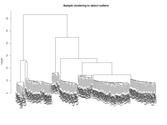
这要是几千个细胞的话，简直一团黑。

powers = c(c(1:10), seq(from = 12, to=30, by=2))
sft = pickSoftThreshold(dataExpr, powerVector=powers, 
                        networkType="signed", verbose=5)

关键就是理解pickSoftThreshold函数及其返回的对象，最佳的beta值就是sft$powerEstimate

par(mfrow = c(1,2))
cex1 = 0.9
# 横轴是Soft threshold (power)，纵轴是无标度网络的评估参数，数值越高，
# 网络越符合无标度特征 (non-scale)
plot(sft$fitIndices[,1], -sign(sft$fitIndices[,3])*sft$fitIndices[,2],
     xlab="Soft Threshold (power)",
     ylab="Scale Free Topology Model Fit,signed R^2",type="n",
     main = paste("Scale independence"))
text(sft$fitIndices[,1], -sign(sft$fitIndices[,3])*sft$fitIndices[,2],
     labels=powers,cex=cex1,col="red")
# 筛选标准。R-square=0.85
abline(h=0.85,col="red")

# Soft threshold与平均连通性
plot(sft$fitIndices[,1], sft$fitIndices[,5],
     xlab="Soft Threshold (power)",ylab="Mean Connectivity", type="n",
     main = paste("Mean connectivity"))
text(sft$fitIndices[,1], sft$fitIndices[,5], labels=powers, 
     cex=cex1, col="red")

power = sft$powerEstimate
softPower  = power
softPower

5

参数beta取值默认是1到30，上述图形的横轴均代表权重参数β，左图纵轴代表对应的网络中log(k)与log(p(k))相关系数的平方。相关系数的平方越高，说明该网络越逼近无网路尺度的分布。右图的纵轴代表对应的基因模块中所有基因邻接函数的均值。最佳的beta值就是sft$powerEstimate，已经被保存到变量了，不需要知道具体是什么，后面的代码都用这个即可，在本例子里面是5。

即使你不理解它，也可以使用代码拿到合适“软阀值（soft thresholding power）”beta进行后续分析。

# 无向网络在power小于15或有向网络power小于30内，没有一个power值可以使
# 无标度网络图谱结构R^2达到0.8，平均连接度较高如在100以上，可能是由于
# 部分样品与其他样品差别太大。这可能由批次效应、样品异质性或实验条件对
# 表达影响太大等造成。可以通过绘制样品聚类查看分组信息和有无异常样品。
# 如果这确实是由有意义的生物变化引起的，也可以使用下面的经验power值。
if (is.na(power)){
  power = ifelse(nSamples<20, ifelse(type == "unsigned", 9, 18),
                 ifelse(nSamples<30, ifelse(type == "unsigned", 8, 16),
                        ifelse(nSamples<40, ifelse(type == "unsigned", 7, 14),
                               ifelse(type == "unsigned", 6, 12))       
                 )
  )
}

power

关键一步：

#一步法网络构建：One-step network construction and module detection##
# power: 上一步计算的软阈值
# maxBlockSize: 计算机能处理的最大模块的基因数量 (默认5000)；
#  4G内存电脑可处理8000-10000个，16G内存电脑可以处理2万个，32G内存电脑可
#  以处理3万个
#  计算资源允许的情况下最好放在一个block里面。
# corType: pearson or bicor
# numericLabels: 返回数字而不是颜色作为模块的名字，后面可以再转换为颜色
# saveTOMs：最耗费时间的计算，存储起来，供后续使用
# mergeCutHeight: 合并模块的阈值，越大模块越少

# type = unsigned

cor <- WGCNA::cor

net = blockwiseModules(dataExpr, power = power, maxBlockSize = nGenes,#nGenes
                       TOMType = "unsigned", minModuleSize = 10,
                       reassignThreshold = 0, mergeCutHeight = 0.25,
                       numericLabels = TRUE, pamRespectsDendro = FALSE,
                       saveTOMs=TRUE, corType = corType, 
                       maxPOutliers=maxPOutliers, loadTOMs=TRUE,
                       saveTOMFileBase = paste0("dataExpr", ".tom"),
                       verbose = 3)

计算过程：

 Calculating module eigengenes block-wise from all genes
   Flagging genes and samples with too many missing values...
    ..step 1
 ..Working on block 1 .
    TOM calculation: adjacency..
    ..will not use multithreading.
     Fraction of slow calculations: 0.000000
    ..connectivity..
    ..matrix multiplication (system BLAS)..
    ..normalization..
    ..done.
   ..saving TOM for block 1 into file dataExpr.tom-block.1.RData
 ....clustering..
 ....detecting modules..
 ....calculating module eigengenes..
 ....checking kME in modules..
     ..removing 109 genes from module 1 because their KME is too low.
     ..removing 17 genes from module 2 because their KME is too low.
 ..merging modules that are too close..
     mergeCloseModules: Merging modules whose distance is less than 0.25
       Calculating new MEs...

我们肯定对这个返回的对象比较感兴趣啦,，挨个查看一下。

table(net$colors)
net$unmergedColors
head(net$MEs)
net$goodSamples
net$goodGenes
net$TOMFiles
net$blockGenes
net$blocks
net$MEsOK
head(net$MEs)
table(net$colors)

 0   1   2   3   4   5 
546 291 111  55  29  17

这里用不同的颜色来代表那些所有的模块，其中灰色默认是无法归类于任何模块的那些基因，如果灰色模块里面的基因太多，那么前期对表达矩阵挑选基因的步骤可能就不太合适。

## 灰色的为**未分类**到模块的基因。
# Convert labels to colors for plotting
moduleLabels = net$colors
moduleColors = labels2colors(moduleLabels)
moduleColors
# Plot the dendrogram and the module colors underneath
# 如果对结果不满意，还可以recutBlockwiseTrees，节省计算时间
plotDendroAndColors(net$dendrograms[[1]], moduleColors[net$blockGenes[[1]]],
                    "Module colors",
                    dendroLabels = FALSE, hang = 0.03,
                    addGuide = TRUE, guideHang = 0.05)

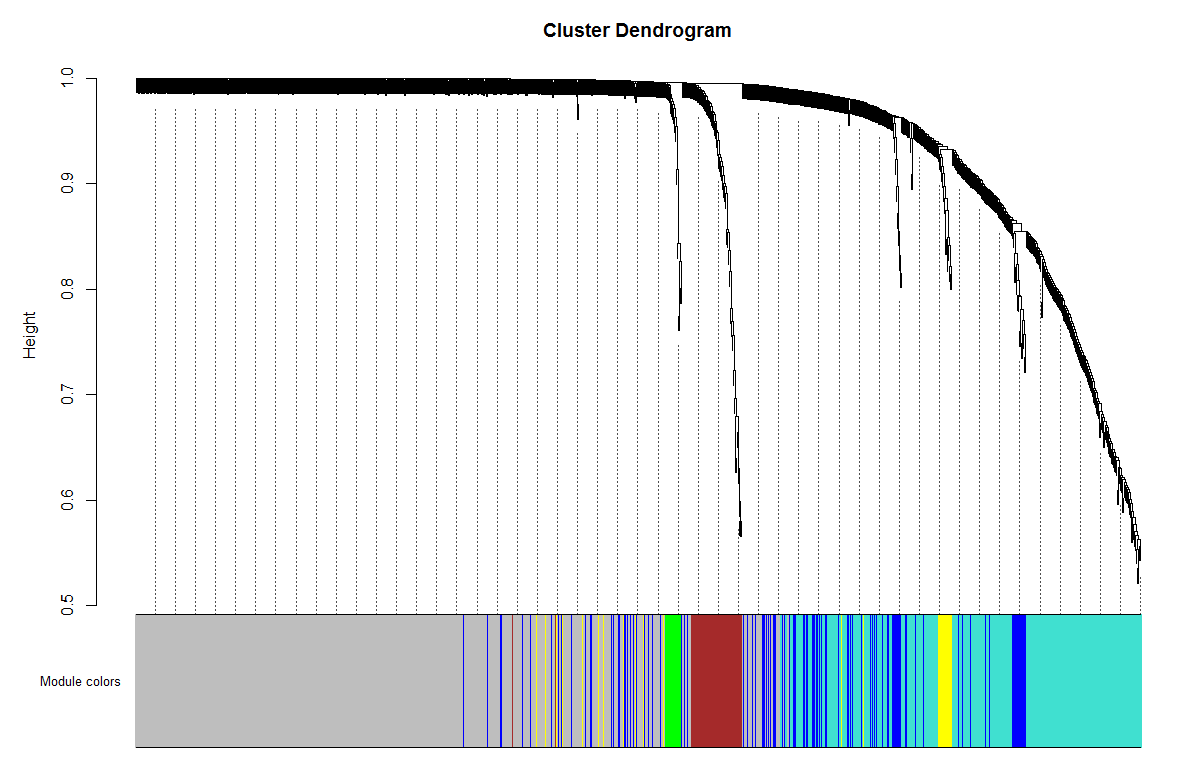
我们这个至少不是全灰的啊。

# module eigengene, 可以绘制线图，作为每个模块的基因表达趋势的展示
MEs = net$MEs

### 不需要重新计算，改下列名字就好
### 官方教程是重新计算的，起始可以不用这么麻烦
MEs_col = MEs
colnames(MEs_col) = paste0("ME", labels2colors(
  as.numeric(str_replace_all(colnames(MEs),"ME",""))))
MEs_col = orderMEs(MEs_col)

# 根据基因间表达量进行聚类所得到的各模块间的相关性图
# marDendro/marHeatmap 设置下、左、上、右的边距
head(MEs_col)
?plotEigengeneNetworks
plotEigengeneNetworks(MEs, "Eigengene adjacency heatmap", 
                      marDendro = c(3,3,2,4),
                      marHeatmap = c(3,4,2,2),
                      plotDendrograms = T,
                      xLabelsAngle = 90)

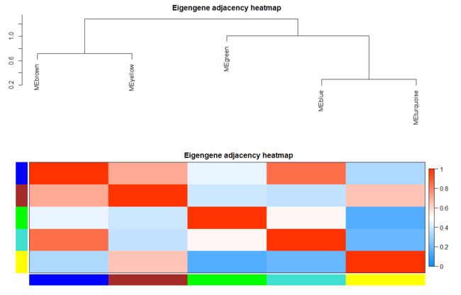
计算每个模块的特征向量基因，为某一特定模块第一主成分基因E。

 计算每个模块的特征向量基因，为某一特定模块第一主成分基因E。代表了该模块内基因表达的整体水平
MEList = moduleEigengenes(dataExpr, colors = dynamicColors)
MEs = MEList$eigengenes
# 计算根据模块特征向量基因计算模块相异度：
MEDiss = 1-cor(MEs);
# Cluster module eigengenes
METree = hclust(as.dist(MEDiss), method = "average");
# Plot the result

plotEigengeneNetworks(MEs, 
                      "Eigengene adjacency heatmap", 
                      marHeatmap = c(3,4,2,2), 
                      plotDendrograms = FALSE, 
                      xLabelsAngle = 90)

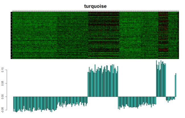
画出指定模块表达量的热图：

which.module="turquoise"; 
ME=mergedMEs[, paste("ME",which.module, sep="")]
par(mfrow=c(2,1), mar=c(0,4.1,4,2.05))
plotMat(t(scale(dataExpr[,moduleColors==which.module ]) ),
        nrgcols=30,rlabels=F,rcols=which.module,
        main=which.module, cex.main=2)
par(mar=c(2,2.3,0.5,0.8))
barplot(ME, col=which.module, main="", cex.main=2,
        ylab="eigengene expression",xlab="array sample")

所有基因模块关系：

load(net$TOMFiles, verbose=T)

## Loading objects:
##   TOM

TOM <- as.matrix(TOM)
TOM[1:4,1:4]
#dim(TOM2)

dissTOM = 1-TOM
# Transform dissTOM with a power to make moderately strong 
# connections more visible in the heatmap
plotTOM = dissTOM^7
# Set diagonal to NA for a nicer plot
diag(plotTOM) = NA
# Call the plot function
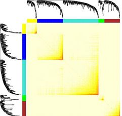
table(moduleColors)
# 这一部分特别耗时，行列同时做层级聚类
TOMplot(plotTOM, net$dendrograms[[1]], moduleColors[net$blockGenes[[1]]], 
        main = "Network heatmap plot, all genes")

由于细胞名称被我们改变了，原来的对象我们要构造表型数据：

Cluster1[1:4,1:4]
mypbmc<- CreateSeuratObject(Cluster1)

mypbmc
mypbmc[["percent.mt"]] <- PercentageFeatureSet(mypbmc, pattern = "^CD")

mypbmc <- FindVariableFeatures(mypbmc, selection.method = "vst", nfeatures = 2000)
mypbmc %>% NormalizeData( normalization.method = "LogNormalize", scale.factor = 10000)%>%
  FindVariableFeatures( selection.method = "vst", nfeatures = 2000) %>%
  ScaleData(features=VariableFeatures(mypbmc),vars.to.regress = "percent.mt")  %>%
  RunPCA(features = VariableFeatures(object = mypbmc)) %>%
  FindNeighbors( dims = 1:10) %>%
  FindClusters( resolution = 0.5) %>%
  BuildClusterTree() %>%
  RunUMAP( dims = 1:10)  -> mypbmc

head([email protected])

head([email protected])
         orig.ident nCount_RNA nFeature_RNA percent.mt RNA_snn_res.0.5 seurat_clusters
1_Cell1           1   477.9562         1030   3.535886               0               0
1_Cell10          1   508.4991         1094   3.107892               0               0
1_Cell11          1   487.7897         1067   3.413325               0               0
1_Cell12          1   464.1321          954   3.189983               0               0
1_Cell13          1   475.1926         1014   3.752087               0               0
1_Cell14          1   502.9780         1072   3.327189               0               0

通过模块与各种表型的相关系数，可以很清楚的挑选自己感兴趣的模块进行下游分析了。

moduleTraitCor_noFP <- cor(mergedMEs, [email protected], use = "p");
moduleTraitPvalue_noFP = corPvalueStudent(moduleTraitCor_noFP, nSamples); 
textMatrix_noFP <- paste(signif(moduleTraitCor_noFP, 2), "\n(", signif(moduleTraitPvalue_noFP, 1), ")", sep = ""); 
par(mar = c(10, 8.5, 3, 3)); 
labeledHeatmap(Matrix = moduleTraitCor_noFP, 
               xLabels = names([email protected]), 
               yLabels = names(mergedMEs), 
               ySymbols = names(mergedMEs), 
               colorLabels = FALSE, 
               colors = blueWhiteRed(50), 
               textMatrix = textMatrix_noFP,
               setStdMargins = FALSE, 
               cex.text = 0.65, 
               zlim = c(-1,1), 
               main = paste("Module-trait relationships"))

根据性状与模块特征向量基因的相关性及pvalue来挖掘与性状相关的模块

library(pheatmap)
cor_ADR <- signif(WGCNA::cor([email protected],mergedMEs,use="p",method="pearson"),5)

p.values <- corPvalueStudent(cor_ADR,nSamples=nrow([email protected]))

pheatmap(cor_ADR,display_numbers = matrix(ifelse(p.values <= 0.01, "**", ifelse(p.values<= 0.05 ,"*"," ")), nrow(p.values)),fontsize=18)

根据基因网络显著性，也就是性状与每个基因表达量相关性在各个模块的均值作为该性状在该模块的显著性，显著性最大的那个模块与该性状最相关：

GS1 <- as.numeric(WGCNA::cor([email protected][,3],dataExpr,use="p",method="pearson"))
# 显著性是绝对值：
GeneSignificance <- abs(GS1)
length(GeneSignificance)
length(mergedColors)
mypbmc
dim(dataExpr)
dim(Cluster1)
dim([email protected])

# 获得该性状在每个模块中的显著性：
ModuleSignificance <- tapply(GeneSignificance,mergedColors,mean,na.rm=T)
ModuleSignificance

     blue     brown     green      grey turquoise    yellow 
0.3817643 0.1335957 0.1147941 0.1291072 0.3386081 0.1243168

寻找与该性状相关的枢纽基因（hub genes）,首先计算基因的内部连接度和模块身份，内部连接度衡量的是基因在模块内部的地位，而模块身份表明基因属于哪个模块。

# 计算每个基因模块内部连接度，也就是基因直接两两加权相关性。
ADJ1=abs(cor(dataExpr,use="p"))^softPower 
# 根据上面结果和基因所属模块信息获得连接度：
# 整体连接度 kTotal，模块内部连接度：kWithin，kOut=kTotal-kWithin， kDiff=kIn-kOut=2*kIN-kTotal 
Alldegrees1=intramodularConnectivity(ADJ1, moduleColors) 
head(Alldegrees1)

          kTotal   kWithin     kOut     kDiff
LYZ    37.799195 35.682342 2.116853 33.565490
S100A9 35.938946 33.908114 2.030833 31.877281
GNLY    5.284786  4.399469 0.885317  3.514152
FTL    44.989900 41.637720 3.352181 38.285539
FTH1   43.791667 41.146166 2.645501 38.500665
S100A8 27.131010 25.587161 1.543848 24.043313

# 注意模块内基于特征向量基因连接度评估模块内其他基因： de ne a module eigengene-based connectivity measure for each gene as the correlation between a the gene expression and the module eigengene
# 如 brown 模块内：kM Ebrown(i) = cor(xi, MEbrown) ， xi is the gene expression pro le of gene i and M Ebrown is the module eigengene of the brown module
# 而 module membership 与内部连接度不同。MM 衡量了基因在全局网络中的位置。
datKME=signedKME(dataExpr, MEs, outputColumnName="MM.")
datKME[1:4,1:4]

# 注意模块内基于特征向量基因连接度评估模块内其他基因： de ne a module eigengene-based connectivity measure for each gene as the correlation between a the gene expression and the module eigengene
# 如 brown 模块内：kM Ebrown(i) = cor(xi, MEbrown) ， xi is the gene expression pro le of gene i and M Ebrown is the module eigengene of the brown module
# 而 module membership 与内部连接度不同。MM 衡量了基因在全局网络中的位置。
datKME=signedKME(dataExpr, MEs, outputColumnName="MM.")
datKME[1:4,1:4]

选择特定模块的基因：

table(moduleColors)
module = "yellow";
# Select module probes
probes = colnames(dataExpr) ## 我们例子里面的probe就是基因名
inModule = (moduleColors==module);
modProbes = probes[inModule]; 
modProbes

 [1] "GIMAP5"  "PPA1"    "CD2"     "AQP3"    "MAL"     "UBAC2"  
 [7] "WTAP"    "SNX3"    "SLFN5"   "ITM2A"   "SUCLG2"  "RWDD1"  
[13] "IL32"    "GIMAP7"  "TRADD"   "CLPP"    "IL7R"    "TOB1"   
[19] "GOLGA7"  "CISH"    "RARRES3" "NOSIP"   "TCF7"    "FXYD5"  
[25] "CUTA"    "CD3D"    "LDHB"    "CD3E"    "RAN"

导出作图文件，主要模块里面的基因直接的相互作用关系信息可以导出到cytoscape,VisANT等网络可视化软件。

## 也是提取指定模块的基因名
# Select the corresponding Topological Overlap
modTOM = TOM[inModule, inModule];
dimnames(modTOM) = list(modProbes, modProbes)
vis = exportNetworkToVisANT(modTOM,
                            file = paste("VisANTInput-", module, ".txt", sep=""),
                            weighted = TRUE,
                            threshold = 0)
?exportNetworkToCytoscape
cyt = exportNetworkToCytoscape(
  modTOM,
  edgeFile = paste("CytoscapeInput-edges-", paste(module, collapse="-"), ".txt", sep=""),
  nodeFile = paste("CytoscapeInput-nodes-", paste(module, collapse="-"), ".txt", sep=""),
  weighted = TRUE,
  threshold = 0.005,
  nodeNames = modProbes, 
  nodeAttr = moduleColors[inModule]
);

单细胞转录组WGCNA到底应该怎么做？

什么是WGCNA

sc-WGCNA

WGCNA in action

你可能感兴趣的:(单细胞转录组WGCNA到底应该怎么做？)