吴恩达机器学习(二十一)—— ex8:Anomaly Detection and Recommender Systems (MATLAB + Python)
- 一、异常检测
-
- 1.1 高斯分布
- 1.2 估计高斯参数
- 1.3 选择阈值 ε ε ε
- 1.4 高维数据集
- 二、推荐系统
-
- 2.1 电影评分数据集
- 2.2 协同滤波学习算法
-
- 2.2.1 协同滤波代价函数
- 2.2.2 协同滤波梯度
- 2.2.3 正则化代价函数
- 2.2.4 正则化梯度
- 2.3 学习电影推荐
-
- 2.3.1 推荐
- 三、MATLAB实现
-
- 3.1 ex8.m
- 3.2 ex8_cofi.m
- 四、Python实现
-
- 4.1 ex8.py
- 4.2 ex8_cofi.py
本次练习对应的基础知识总结 → \rightarrow →异常检测和推荐系统。
本次练习对应的文档说明和提供的MATLAB代码 → \rightarrow → 提取码:7g7b 。
本次练习对应的完整代码实现(MATLAB + Python版本) → \rightarrow →Github链接。
一、异常检测
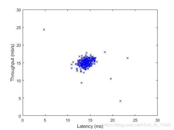
在本练习中,我们将实现异常检测算法以检测服务器计算机中的异常行为。该特征为每个服务器响应的吞吐量(mb/s)和延迟(ms)。当我们的服务器正在运行时,我们收集了 m = 307 m = 307 m=307个它们行为方式的样本,因此有一个未标记的数据集 { x ( 1 ) , x ( 2 ) , . . . , x ( m ) } \{x^{(1)},x^{(2)},...,x^{(m)}\} { x(1),x(2),...,x(m)}。我们认为绝大多数的样本是“正常的”(非异常的),即服务器正常运行,但在该数据集中也可能有一些服务器异常运行。
我们将使用高斯模型来检测数据集中的异常样本。我们将首先从2D数据集上开始,允许可视化算法正在进行的内容。在该数据集上,我们将拟合高斯分布,然后找到具有非常低的概率的值,可以被视为异常。之后,我们将应用异常检测算法于具有很多维度的较大数据集。我们将在这部分练习中使用ex8.m。
ex8.m的第一部分将可视化数据集,如图1所示。
1.1 高斯分布
要进行异常检测,我们将首先需要使模型去拟合数据的分布。
给定训练集 { x ( 1 ) , x ( 2 ) , . . . , x ( m ) } \{x^{(1)},x^{(2)},...,x^{(m)}\} { x(1),x(2),...,x(m)}(其中 x ( i ) ∈ R n x^{(i)}∈R^{n} x(i)∈Rn),我们想要估计每个特征 x ( i ) x^{(i)} x(i)的高斯分布。对于每个特征 i = 1 , . . . , n i = 1,...,n i=1,...,n,我们需要找到参数 μ i μ_{i} μi和 σ i 2 \sigma_{i}^{2} σi2拟合第 i i i维的数据 { x i ( 1 ) , x i ( 2 ) , . . . , x i ( m ) } \{x_{i}^{(1)},x_{i}^{(2)},...,x_{i}^{(m)}\} { xi(1),xi(2),...,xi(m)}(每个样本的第 i i i个维度)。
高斯分布由下式给出 p ( x ; μ , σ 2 ) = 1 2 π σ e ( − ( x − μ ) 2 2 σ 2 ) p(x; \mu , \sigma ^{2})=\frac{1}{\sqrt{2\pi \sigma }}e^{(-\frac{(x-\mu )^{2}}{2\sigma ^{2}})} p(x;μ,σ2)=2πσ1e(−2σ2(x−μ)2)其中, μ μ μ是均值, σ 2 \sigma ^{2} σ2是方差。
1.2 估计高斯参数
我们可以使用以下等式估计第 i i i个特征的参数 ( μ i , σ i 2 ) (μ_{i},\sigma_{i} ^{2}) (μi,σi2)。要计算均值,我们将使用 μ i = 1 m ∑ j = 1 m x i ( j ) \mu_{i} =\frac{1}{m}\sum ^{m}_{j=1}x_{i}^{(j)} μi=m1j=1∑mxi(j)对于方差。我们使用 σ i 2 = 1 m ∑ j = 1 m ( x i ( j ) − μ i ) 2 \sigma_{i} ^{2}=\frac{1}{m}\sum ^{m}_{j=1}(x_{i} ^{(j)}-\mu_{i} )^{2} σi2=m1j=1∑m(xi(j)−μi)2 我们的任务是完成 estimateGaussian.m中的代码。此函数输入数据矩阵 X X X,应该输出一个保存所有 n n n个特征均值的n维向量 μ \mu μ,以及输出另一个保存所有特征方差的n维向量 σ 2 \sigma^{2} σ2。我们可以在每个特征和每个训练样本中使用for循环实现这一点(向量化实现可能更有效)。要注意的是,在MATLAB中,当计算 σ i 2 \sigma_{i}^{2} σi2时,var函数(默认情况下)使用 1 m − 1 \frac{1}{m-1} m−11,而不是 1 m \frac{1}{m} m1。
完成estimateGaussian.m需要填写以下代码:
mu = mean(X)';
%var normalizes V by N-1 if N>1,where N is the sample size.
% sigma2 = var(X) * (n -1) / n;
for i = 1:n
    X(:,i) = X(:,i) - mu(i);
end
sigma2 = 1 / m * sum(X .^2)';
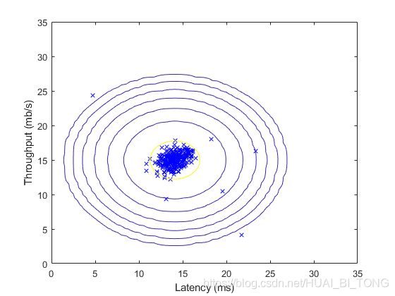
完成estimateGaussian.m的代码后,ex8.m的下一部分将可视化拟合高斯分布的轮廓。我们可以得到图2。从图中可以看到大多数样本在具有最高概率的区域中,而异常样本在具有较低概率的区域中。
1.3 选择阈值 ε ε ε
现在我们已经估计了高斯参数,可以研究在该分布的情况下哪个样本具有非常高的概率,哪个样本具有非常低的概率。低概率样本更可能是我们数据集中的异常点。一种确定哪个样本是异常的方法是基于交叉验证集来选择阈值。在这一部分的练习中,我们将使用F1分数在交叉验证集上实现算法,以选择阈值 ε ε ε。
我们现在应该完成selectThreshold.m中的代码。为此,我们将使用交叉验证集 { ( x c v ( 1 ) , y c v ( 1 ) ) \{(x_{cv}^{(1)},y_{cv}^{(1)}) { (xcv(1),ycv(1)),…, ( x c v ( m c v ) , y c v ( m c v ) ) } (x_{cv}^{(m_{cv})},y_{cv}^{(m_{cv})})\} (xcv(mcv),ycv(mcv))},其中标签 y = 1 y = 1 y=1对应于异常样本, y = 0 y = 0 y=0对应于正常样本。对于每个交叉验证样本,我们将计算 p ( x c v ( i ) ) p(x_{cv}^{(i)}) p(xcv(i))。所有这些概率 p ( x c v ( 1 ) ) p(x_{cv}^{(1)}) p(xcv(1)),…, p ( x c v ( m c v ) ) p(x_{cv}^{(m_{cv})}) p(xcv(mcv))的向量在向量pval中并传递给selectThreshold.m,相应的标签 y c v ( 1 ) y_{cv}^{(1)} ycv(1),…, y c v ( m c v ) y_{cv}^{(m_{cv})} ycv(mcv)在向量yval中并传递给相同的函数。
函数selectThreshold.m应该返回两个值,第一个是所选的阈值 ε ε ε。如果样本 x x x具有较低的概率 p ( x ) < ε p(x)<ε p(x)<ε,则认为它是异常的。该函数还应该返回F1分数,它说明在给定一定的阈值时,寻找异常方面做得效果如何。对于许多不同的 ε ε ε值,我们将通过计算当前阈值正确和错误分类样本的多少来计算生成的F1分数。
使用准确率( p r e c prec prec)和召回率( r e c rec rec)计算F1分数: F 1 = 2 ⋅ p r e c ⋅ r e c p r e c + r e c F_{1} = \frac{2 \cdot prec \cdot rec}{prec+rec} F1=prec+rec2⋅prec⋅rec由下式可计算准确率和召回率: p r e c = t p t p + f p prec=\frac{tp}{tp+fp} prec=tp+fptp r e c = t p t p + f n rec=\frac{tp}{tp+fn} rec=tp+fntp其中, • t p tp tp是真阳性的数量:地面真值标签表示它是一个异常,我们的算法将其正确分类为异常。
• f p fp fp是假阳性的数量:地面真值标签表示它不是一个异常,但我们的算法错误地将其分类为异常。
• f n fn fn是假阴性的数量:地面真值标签表示它是一个异常,但我们的算法错误地将其分类为不是异常的。
在提供的代码selectThreshold.m中,已经存在一个循环,它将尝试许多不同的 ε ε ε值,并根据F1分数选择最佳 ε ε ε。
我们现在应该在selectThreshold.m中完成代码。我们可以在所有交叉验证样本中使用for循环实现F1分数的计算(计算 t p tp tp, f p fp fp, f n fn fn的值)。
完成selectThreshold.m需要在for循环中填写以下代码:
    cvPredictions = (pval < epsilon);
    tp = sum((cvPredictions == 1) & (yval == 1));%cvPredictions == 1表示pvalepsilon,预测为正常(阴性)

    prec = tp/(tp+fp);
    rec = tp/(tp+fn);

    F1 = (2*prec*rec)/(prec+rec);
完成selectThreshold.m中的代码后,运行ex8.m,我们应该看到epsilon的值约为8.99e-05,且ex8.m的下一步将运行我们的异常检测代码并圈出图中的异常点(如图3)。
Best epsilon found using cross-validation: 8.990853e-05
Best F1 on Cross Validation Set:  0.875000
   (you should see a value epsilon of about 8.99e-05)
   (you should see a Best F1 value of  0.875000)

1.4 高维数据集
脚本ex8.m的最后一部分将在更现实、更难的数据集中运行我们实现的异常检测算法。在此数据集中,每个样本由11个特征描述,捕获计算服务器的更多属性。
该脚本将使用我们的代码来估计高斯参数( μ i μ_{i} μi和 σ i 2 \sigma_{i} ^{2} σi2),求出我们估计高斯参数的训练数据 X X X的概率,并在交叉验证集Xval上执行。最后,它将使用 selectThreshold 找到最佳阈值 ε ε ε。我们应该看到一个值约1.38e-18的epsilon,并找到117个异常。
Best epsilon found using cross-validation: 1.377229e-18
Best F1 on Cross Validation Set:  0.615385
   (you should see a value epsilon of about 1.38e-18)
   (you should see a Best F1 value of 0.615385)
# Outliers found: 117
二、推荐系统
在这一部分的练习中,我们将实现协同过滤学习算法,并将其应用于电影评分的数据集,这个数据集包含范围为1-5的评分。该数据集具有 n u = 943 n_{u} = 943 nu=943个用户, n m = 1682 n_{m} = 1682 nm=1682部电影。在这部分练习中,我们将使用脚本ex8_cofi.m。
在本练习的下一部分中,我们将实现 cofiCostFunc.m的函数来计算协同滤波的目标函数和梯度。在实现代价函数和梯度后,我们将使用fmincg.m来学习协同滤波的参数。
2.1 电影评分数据集
脚本ex8_cofi.m的第一部分将加载数据集ex8 movies.mat,在 MATLAB环境中提供变量 Y Y Y和 R R R。
矩阵 Y Y Y(一个num movies×num movies矩阵)存储评分 y ( i , j ) y^{(i,j)} y(i,j)(从1到5)。矩阵 R R R是二进制值指示符矩阵,其中如果用户 j j j给电影 i i i评过分,则 R ( i , j ) = 1 R(i,j)= 1 R(i,j)=1,否则 R ( i , j ) = 0 R(i,j)= 0 R(i,j)=0。协同滤波的目标是预测用户尚未评分的电影评分,即 R ( i , j ) = 0 R(i,j)= 0 R(i,j)=0的条目。这将允许我们给用户推荐具有最高预测评分的电影。
为了有助于了解矩阵 Y Y Y,脚本ex8_cofi.m将计算第一部电影(Toy Story)的平均电影评分,并将平均评分输出到屏幕。
在整个练习中,我们还将使用矩阵 X X X和 T h e t a Theta Theta: X = [ − ( x ( 1 ) ) T − − ( x ( 2 ) ) T − ⋮ − ( x ( n m ) ) T − ] , T h e t a = [ − ( θ ( 1 ) ) T − − ( θ ( 2 ) ) T − ⋮ − ( θ ( n u ) ) T − ] X=\begin{bmatrix} -(x^{(1)})^{T}-\\ -(x^{(2)})^{T}-\\ \vdots \\ -(x^{(n_m)})^{T}- \end{bmatrix},Theta=\begin{bmatrix} -(\theta^{(1)})^{T}-\\ -(\theta^{(2)})^{T}-\\ \vdots \\ -(\theta^{(n_u)})^{T}- \end{bmatrix} X=⎣⎢⎢⎢⎡−(x(1))T−−(x(2))T−⋮−(x(nm))T−⎦⎥⎥⎥⎤,Theta=⎣⎢⎢⎢⎡−(θ(1))T−−(θ(2))T−⋮−(θ(nu))T−⎦⎥⎥⎥⎤对于第 i i i部电影, X X X的第 i i i行对应于特征向量 x ( i ) x^{(i)} x(i), T h e t a Theta Theta的第 j j j行对应于参数向量 θ ( j ) θ^{(j)} θ(j)。 x ( i ) x^{(i)} x(i)和 θ ( j ) θ^{(j)} θ(j)都是 n n n维向量。出于本练习的目的,我们将使用 n = 100 n = 100 n=100,因此, x ( i ) ∈ R 100 x^{(i)}∈R^{100} x(i)∈R100和 θ ( j ) ∈ R 100 θ^{(j)}∈R^{100} θ(j)∈R100。相应地, X X X是 n m × 100 n_{m}×100 nm×100的矩阵,并且 T h e t a Theta Theta是 n u × 100 n_{u}×100 nu×100的矩阵。
2.2 协同滤波学习算法
现在,我们将开始实现协同滤波学习算法。我们将首先实现代价函数(没有正则化)。
在电影推荐的设置中,协同滤波算法考虑了一组 n n n维参数向量 x ( 1 ) x^{(1)} x(1),…, x ( n m ) x^{(n_{m})} x(nm)和 θ ( 1 ) θ^{(1)} θ(1),…, θ ( n u ) θ^{(n_{u})} θ(nu),其中模型预测用户 j j j为电影 i i i的评分为 y ( i , j ) = ( θ ( j ) ) T x ( i ) y^{(i,j)} =(θ^{(j)})^{T}x^{(i)} y(i,j)=(θ(j))Tx(i)。给定一些由某些用户在某些电影上产生的评分组成的数据集,希望学习参数向量 x ( 1 ) x^{(1)} x(1),…, x ( n m ) x^{(n_{m})} x(nm), θ ( 1 ) θ^{(1)} θ(1),…, θ ( n u ) θ^{(n_{u})} θ(nu)产生的最佳拟合(最小化平方误差)。
我们将在cofiCostFunc.m中填写代码,以计算协同滤波的代价函数和梯度。请注意,函数的参数是 X X X和 T h e t a Theta Theta。为了使用诸如fmincg之类的现成最小化库,已经设置代价函数以将参数展开到单个向量param中。我们以前在神经网络编程练习中使用过相同的向量展开方法。
2.2.1 协同滤波代价函数
协同滤波代价函数(没有正则化)由下式给出 J ( x ( 1 ) , . . . , x ( n m ) , θ ( 1 ) , . . . , θ ( n u ) ) = 1 2 ∑ ( i , j ) : r ( i , j ) = 1 ( ( θ ( j ) ) T x ( i ) − y ( i , j ) ) 2 J(x^{(1)},...,x^{(n_{m})},\theta^{(1)},...,\theta^{(n_{u})})= \frac{1}{2}\sum _{(i,j):r(i,j)=1}\left ( (\theta^{(j)})^{T}x^{(i)}-y^{(i,j)}\right )^{2} J(x(1),...,x(nm),θ(1),...,θ(nu))=21(i,j):r(i,j)=1∑((θ(j))Tx(i)−y(i,j))2 我们现在应该修改cofiCostFunc.m,以在变量 J J J中返回此代价。要注意的是,只有当 R ( i , j ) = 1 R(i,j)= 1 R(i,j)=1时,我们才应该累积用户 j j j和电影 i i i的代价。
完成cofiCostFunc.m中的代价函数部分需要填写以下代码:
%代价函数
J = sum(sum(((X*Theta').*R-Y).^2))/2;
完成函数后,脚本ex8_cofi.m将运行我们的代价函数。我们应该看到22.22的输出。
Cost at loaded parameters: 22.224604
(this value should be about 22.22)
2.2.2 协同滤波梯度
现在,我们应该实现梯度(没有正则化)。具体来说,我们应该在cofiCostFunc.m中填写代码,以返回变量 X _ g r a d X\_grad X_grad和 T h e t a _ g r a d Theta\_grad Theta_grad。注意, X _ g r a d X\_grad X_grad应是与 X X X相同尺寸的矩阵,类似地, T h e t a _ g r a d Theta\_grad Theta_grad是与 T h e t a Theta Theta相同尺寸的矩阵。代价函数的梯度由下式给出: ∂ J ∂ x k ( i ) = ∑ j : r ( i , j ) = 1 ) ( ( θ ( j ) ) T x ( i ) − y ( i , j ) ) θ k ( j ) \frac{\partial J}{\partial x^{(i)}_{k}}= \sum _{j:r(i,j)=1)}\left ( (\theta^{(j)})^{T}x^{(i)}-y^{(i,j)}\right )\theta_{k}^{(j)} ∂xk(i)∂J=j:r(i,j)=1)∑((θ(j))Tx(i)−y(i,j))θk(j) ∂ J ∂ θ k ( j ) = ∑ i : r ( i , j ) = 1 ) ( ( θ ( j ) ) T x ( i ) − y ( i , j ) ) x k ( i ) \frac{\partial J}{\partial \theta ^{(j)}_{k}}= \sum _{i:r(i,j)=1)}\left ( (\theta^{(j)})^{T}x^{(i)}-y^{(i,j)}\right )x_{k}^{(i)} ∂θk(j)∂J=i:r(i,j)=1)∑((θ(j))Tx(i)−y(i,j))xk(i) 要注意的是,该函数通过将它们展开到单个向量中的两组变量返回梯度。
完成cofiCostFunc.m中的梯度部分需要填写以下代码:
%梯度
for i=1:num_movies
    idx = find(R(i,:)==1);
    Theta_temp = Theta(idx,:);
    Y_temp = Y(i,idx);
    X_grad(i,:)= (X(i,:)*Theta_temp'-Y_temp)*Theta_temp;
end

for j=1:num_users
    idx = find(R(:,j)==1);
    X_temp = X(idx,:);
    Y_temp = Y(idx,j);
    Theta_grad(j,:) = ((X_temp*Theta(j,:)'-Y_temp))'*X_temp;
end
完成代码来计算梯度后,脚本ex8_cofi.m将运行梯度检查(checkCostFunction)以数值方式检查我们的梯度实现。如果我们的实现是正确的,则会发现分析和数值梯度紧密配合。
Checking Gradients (without regularization) ...
    5.5335    5.5335
    3.6186    3.6186
    5.4422    5.4422
   -1.7312   -1.7312
    4.1196    4.1196
   -1.4833   -1.4833
   -6.0734   -6.0734
    2.3490    2.3490
    7.6341    7.6341
    1.8651    1.8651
    4.1192    4.1192
   -1.5834   -1.5834
    1.2828    1.2828
   -6.1573   -6.1573
    1.6628    1.6628
    1.1686    1.1686
    5.5630    5.5630
    0.3050    0.3050
    4.6442    4.6442
   -1.6691   -1.6691
   -2.1505   -2.1505
   -3.6832   -3.6832
    3.4067    3.4067
   -4.0743   -4.0743
    0.5567    0.5567
   -2.1056   -2.1056
    0.9168    0.9168

The above two columns you get should be very similar.
(Left-Your Numerical Gradient, Right-Analytical Gradient)

If your cost function implementation is correct, then
the relative difference will be small (less than 1e-9).

Relative Difference: 1.7768e-12
2.2.3 正则化代价函数
通过正则化进行协同滤波的代价函数由下式给出
J ( x ( 1 ) , . . . , x ( n m ) , θ ( 1 ) , . . . , θ ( n u ) ) = 1 2 ∑ ( i , j ) : r ( i , j ) = 1 ( ( θ ( j ) ) T x ( i ) − y ( i , j ) ) 2 + λ 2 ∑ i = 1 n m ∑ k = 1 n ( x k ( i ) ) ) 2 + λ 2 ∑ j = 1 n u ∑ k = 1 n ( θ k ( j ) ) ) 2 J(x^{(1)},...,x^{(n_{m})},\theta^{(1)},...,\theta^{(n_{u})})= \frac{1}{2}\sum _{(i,j):r(i,j)=1}\left ( (\theta^{(j)})^{T}x^{(i)}-y^{(i,j)}\right )^{2}+\frac{\lambda }{2}\sum ^{n_{m}}_{i=1}\sum ^{n}_{k=1}\left ( x_{k}^{(i)}) \right )^{2}+\frac{\lambda }{2}\sum ^{n_{u}}_{j=1}\sum ^{n}_{k=1}\left ( \theta_{k}^{(j)}) \right )^{2} J(x(1),...,x(nm),θ(1),...,θ(nu))=21(i,j):r(i,j)=1∑((θ(j))Tx(i)−y(i,j))2+2λi=1∑nmk=1∑n(xk(i)))2+2λj=1∑nuk=1∑n(θk(j)))2 我们现在应该将正则化添加到我们的代价函数 J J J的原始计算中。
添加正则化到我们的代价函数部分,需要修改cofiCostFunc.m中的代价函数部分代码为:
%代价函数
J = sum(sum(((X*Theta').*R-Y).^2))/2;
J = J + sum(sum(Theta.^2))*lambda/2 + sum(sum(X.^2))*lambda/2;
完成后,脚本ex8_cofi.m将运行我们的正则化代价函数,并且我们应该看到大约31.34的成本。
Cost at loaded parameters (lambda = 1.5): 31.344056
(this value should be about 31.34)
2.2.4 正则化梯度
现在我们已经实现了正则化代价函数,应该继续实现正则化梯度。我们应该在cofiCostFunc.m中添加正则化项来返回正则化梯度。正则化代价函数的梯度由下式给出: ∂ J ∂ x k ( i ) = ∑ j : r ( i , j ) = 1 ) ( ( θ ( j ) ) T x ( i ) − y ( i , j ) ) θ k ( j ) + λ x k ( i ) \frac{\partial J}{\partial x^{(i)}_{k}}= \sum _{j:r(i,j)=1)}\left ( (\theta^{(j)})^{T}x^{(i)}-y^{(i,j)}\right )\theta_{k}^{(j)}+\lambda x^{(i)}_{k} ∂xk(i)∂J=j:r(i,j)=1)∑((θ(j))Tx(i)−y(i,j))θk(j)+λxk(i) ∂ J ∂ θ k ( j ) = ∑ i : r ( i , j ) = 1 ) ( ( θ ( j ) ) T x ( i ) − y ( i , j ) ) x k ( i ) + λ θ k ( j ) \frac{\partial J}{\partial \theta ^{(j)}_{k}}= \sum _{i:r(i,j)=1)}\left ( (\theta^{(j)})^{T}x^{(i)}-y^{(i,j)}\right )x_{k}^{(i)}+\lambda \theta ^{(j)}_{k} ∂θk(j)∂J=i:r(i,j)=1)∑((θ(j))Tx(i)−y(i,j))xk(i)+λθk(j) 这意味着我们只需要将 λ x ( i ) \lambda x^{(i)} λx(i)添加到之前定义的变量X_grad(i,:)中,并将 λ θ ( j ) \lambda \theta ^{(j)} λθ(j)添加到之前定义的变量Theta_grad(j,:)中。
添加正则化到我们的梯度部分,需要修改cofiCostFunc.m中的梯度部分代码为:
%梯度
for i=1:num_movies
    idx = find(R(i,:)==1);
    Theta_temp = Theta(idx,:);
    Y_temp = Y(i,idx);
    X_grad(i,:)= (X(i,:)*Theta_temp'-Y_temp)*Theta_temp;
    X_grad(i,:) = X_grad(i,:)+lambda*X(i,:);
end

for j=1:num_users
    idx = find(R(:,j)==1);
    X_temp = X(idx,:);
    Y_temp = Y(idx,j);
    Theta_grad(j,:) = ((X_temp*Theta(j,:)'-Y_temp))'*X_temp;
    Theta_grad(j,:) = Theta_grad(j,:) + lambda*Theta(j,:);
end
完成了计算梯度的代码后,脚本ex8_cofi.m将运行另一个梯度检查(checkCostFunction)以数值地方式检查我们实现的梯度。
Checking Gradients (with regularization) ...
    2.2223    2.2223
    0.7968    0.7968
   -3.2924   -3.2924
   -0.7029   -0.7029
   -4.2016   -4.2016
    3.5969    3.5969
    0.8859    0.8859
    1.0523    1.0523
   -7.8499   -7.8499
    0.3904    0.3904
   -0.1347   -0.1347
   -2.3656   -2.3656
    2.1066    2.1066
    1.6703    1.6703
    0.8519    0.8519
   -1.0380   -1.0380
    2.6537    2.6537
    0.8114    0.8114
   -0.8604   -0.8604
   -0.5884   -0.5884
   -0.7108   -0.7108
   -4.0652   -4.0652
    0.2494    0.2494
   -4.3484   -4.3484
   -3.6167   -3.6167
   -4.1277   -4.1277
   -3.2439   -3.2439

The above two columns you get should be very similar.
(Left-Your Numerical Gradient, Right-Analytical Gradient)

If your cost function implementation is correct, then
the relative difference will be small (less than 1e-9).

Relative Difference: 1.82991e-12
2.3 学习电影推荐
实现协同滤波的代价函数和梯度之后,我们现在可以开始训练算法来为自己制作电影推荐。在ex8_cofi.m脚本的下一部分中,我们可以输入自己喜欢的电影,以便之后在运行算法时,可以获得自己的电影推荐!提供的文本已经根据一些人的喜好填写了一些值,但我们应该根据自己的喜好进行改变。在文件movie_idx.txt中通过了所有电影及其编号的数据集。
2.3.1 推荐
在数据集中添加了额外的评分后,脚本将继续训练协同滤波模型,这将学习参数 X X X和 T h e t a Theta Theta。为了预测用户 i i i对电影 i i i的评分,我们需要计算 ( θ ( j ) ) T x ( i ) ) (\theta ^{(j)})^{T}x ^{(i)}) (θ(j))Tx(i))。脚本的下一部分计算所有电影和用户的评分,并根据脚本前面输入的评分,显示其推荐的电影。要注意的是,由于不同的随机初始化,我们可能会获得不同的预测。
Top recommendations for you:
Predicting rating 5.0 for movie Great Day in Harlem, A (1994)
Predicting rating 5.0 for movie Saint of Fort Washington, The (1993)
Predicting rating 5.0 for movie Someone Else's America (1995)
Predicting rating 5.0 for movie Santa with Muscles (1996)
Predicting rating 5.0 for movie Entertaining Angels: The Dorothy Day Story (1996)
Predicting rating 5.0 for movie Aiqing wansui (1994)
Predicting rating 5.0 for movie Prefontaine (1997)
Predicting rating 5.0 for movie They Made Me a Criminal (1939)
Predicting rating 5.0 for movie Marlene Dietrich: Shadow and Light (1996)
Predicting rating 5.0 for movie Star Kid (1997)


Original ratings provided:
Rated 4 for Toy Story (1995)
Rated 3 for Twelve Monkeys (1995)
Rated 5 for Usual Suspects, The (1995)
Rated 4 for Outbreak (1995)
Rated 5 for Shawshank Redemption, The (1994)
Rated 3 for While You Were Sleeping (1995)
Rated 5 for Forrest Gump (1994)
Rated 2 for Silence of the Lambs, The (1991)
Rated 4 for Alien (1979)
Rated 5 for Die Hard 2 (1990)
Rated 5 for Sphere (1998)
三、MATLAB实现
3.1 ex8.m
%% Machine Learning Online Class
%  Exercise 8 | Anomaly Detection and Collaborative Filtering
%
%  Instructions
%  ------------
%
%  This file contains code that helps you get started on the
%  exercise. You will need to complete the following functions:
%
%     estimateGaussian.m
%     selectThreshold.m
%     cofiCostFunc.m
%
%  For this exercise, you will not need to change any code in this file,
%  or any other files other than those mentioned above.
%

%% Initialization
clear ; close all; clc

%% ================== Part 1: Load Example Dataset  ===================
%  We start this exercise by using a small dataset that is easy to
%  visualize.
%
%  Our example case consists of 2 network server statistics across
%  several machines: the latency and throughput of each machine.
%  This exercise will help us find possibly faulty (or very fast) machines.
%

fprintf('Visualizing example dataset for outlier detection.\n\n');

%  The following command loads the dataset. You should now have the
%  variables X, Xval, yval in your environment
load('ex8data1.mat');

%  Visualize the example dataset
plot(X(:, 1), X(:, 2), 'bx');
axis([0 30 0 30]);
xlabel('Latency (ms)');
ylabel('Throughput (mb/s)');

fprintf('Program paused. Press enter to continue.\n');
pause


%% ================== Part 2: Estimate the dataset statistics ===================
%  For this exercise, we assume a Gaussian distribution for the dataset.
%
%  We first estimate the parameters of our assumed Gaussian distribution,
%  then compute the probabilities for each of the points and then visualize
%  both the overall distribution and where each of the points falls in
%  terms of that distribution.
%
fprintf('Visualizing Gaussian fit.\n\n');

%  Estimate my and sigma2
%  通过数据集估计参数
[mu sigma2] = estimateGaussian(X);%estimateGaussian(X)使用X中的数据估计高斯分布的参数

%  Returns the density of the multivariate normal at each data point (row) of X
%  训练训练集模型
p = multivariateGaussian(X, mu, sigma2);%multivariateGaussian()计算多元高斯分布的概率密度函数

%  Visualize the fit
visualizeFit(X,  mu, sigma2);
xlabel('Latency (ms)');
ylabel('Throughput (mb/s)');

fprintf('Program paused. Press enter to continue.\n');
pause;

%% ================== Part 3: Find Outliers ===================
%  Now you will find a good epsilon threshold using a cross-validation set
%  probabilities given the estimated Gaussian distribution
%

%  训练交叉验证集模型(用来选择最终的epsilon)
pval = multivariateGaussian(Xval, mu, sigma2);

[epsilon F1] = selectThreshold(yval, pval);%selectThreshold()找到用于选择异常值的最佳阈值(epsilon)
fprintf('Best epsilon found using cross-validation: %e\n', epsilon);
fprintf('Best F1 on Cross Validation Set:  %f\n', F1);
fprintf('   (you should see a value epsilon of about 8.99e-05)\n');
fprintf('   (you should see a Best F1 value of  0.875000)\n\n');

%  Find the outliers in the training set and plot the
outliers = find(p < epsilon);%异常值

%  Draw a red circle around those outliers
visualizeFit(X,  mu, sigma2);
xlabel('Latency (ms)');
ylabel('Throughput (mb/s)');
hold on
plot(X(outliers, 1), X(outliers, 2), 'ro', 'LineWidth', 2, 'MarkerSize', 10);
hold off

fprintf('Program paused. Press enter to continue.\n');
pause;

%% ================== Part 4: Multidimensional Outliers ===================
%  We will now use the code from the previous part and apply it to a
%  harder problem in which more features describe each datapoint and only
%  some features indicate whether a point is an outlier.
%

%  Loads the second dataset. You should now have the
%  variables X, Xval, yval in your environment
load('ex8data2.mat');

%  Apply the same steps to the larger dataset
[mu sigma2] = estimateGaussian(X);

%  Training set
p = multivariateGaussian(X, mu, sigma2);

%  Cross-validation set
pval = multivariateGaussian(Xval, mu, sigma2);

%  Find the best threshold
[epsilon F1] = selectThreshold(yval, pval);

fprintf('Best epsilon found using cross-validation: %e\n', epsilon);
fprintf('Best F1 on Cross Validation Set:  %f\n', F1);
fprintf('   (you should see a value epsilon of about 1.38e-18)\n');
fprintf('   (you should see a Best F1 value of 0.615385)\n');
fprintf('# Outliers found: %d\n\n', sum(p < epsilon));
3.2 ex8_cofi.m
%% Machine Learning Online Class
%  Exercise 8 | Anomaly Detection and Collaborative Filtering
%
%  Instructions
%  ------------
%
%  This file contains code that helps you get started on the
%  exercise. You will need to complete the following functions:
%
%     estimateGaussian.m
%     selectThreshold.m
%     cofiCostFunc.m
%
%  For this exercise, you will not need to change any code in this file,
%  or any other files other than those mentioned above.
%

%% =============== Part 1: Loading movie ratings dataset ================
%  You will start by loading the movie ratings dataset to understand the
%  structure of the data.
%
fprintf('Loading movie ratings dataset.\n\n');

%  Load data
load ('ex8_movies.mat');

%  Y is a 1682x943 matrix, containing ratings (1-5) of 1682 movies on
%  943 users
%
%  R is a 1682x943 matrix, where R(i,j) = 1 if and only if user j gave a
%  rating to movie i

%  From the matrix, we can compute statistics like average rating.
fprintf('Average rating for movie 1 (Toy Story): %f / 5\n\n', mean(Y(1, R(1, :))));%Y(1, R(1, :)):R中第一行为1的元素对应的Y中第一行的元素

%  We can "visualize" the ratings matrix by plotting it with imagesc
imagesc(Y);
ylabel('Movies');
xlabel('Users');

fprintf('\nProgram paused. Press enter to continue.\n');
pause;

%% ============ Part 2: Collaborative Filtering Cost Function ===========
%  You will now implement the cost function for collaborative filtering.
%  To help you debug your cost function, we have included set of weights
%  that we trained on that. Specifically, you should complete the code in
%  cofiCostFunc.m to return J.

%  Load pre-trained weights (X, Theta, num_users, num_movies, num_features)
load ('ex8_movieParams.mat');

%  Reduce the data set size so that this runs faster
num_users = 4; num_movies = 5; num_features = 3;
X = X(1:num_movies, 1:num_features);%X为num_movies乘num_features
Theta = Theta(1:num_users, 1:num_features);
Y = Y(1:num_movies, 1:num_users);
R = R(1:num_movies, 1:num_users);

%  Evaluate cost function
J = cofiCostFunc([X(:) ; Theta(:)], Y, R, num_users, num_movies, num_features, 0);

fprintf(['Cost at loaded parameters: %f '...
         '\n(this value should be about 22.22)\n'], J);

fprintf('\nProgram paused. Press enter to continue.\n');
pause;


%% ============== Part 3: Collaborative Filtering Gradient ==============
%  Once your cost function matches up with ours, you should now implement
%  the collaborative filtering gradient function. Specifically, you should
%  complete the code in cofiCostFunc.m to return the grad argument.
%
fprintf('\nChecking Gradients (without regularization) ... \n');

%  Check gradients by running checkNNGradients
checkCostFunction;

fprintf('\nProgram paused. Press enter to continue.\n');
pause;


%% ========= Part 4: Collaborative Filtering Cost Regularization ========
%  Now, you should implement regularization for the cost function for
%  collaborative filtering. You can implement it by adding the cost of
%  regularization to the original cost computation.
%

%  Evaluate cost function
J = cofiCostFunc([X(:) ; Theta(:)], Y, R, num_users, num_movies, num_features, 1.5);

fprintf(['Cost at loaded parameters (lambda = 1.5): %f '...
         '\n(this value should be about 31.34)\n'], J);

fprintf('\nProgram paused. Press enter to continue.\n');
pause;


%% ======= Part 5: Collaborative Filtering Gradient Regularization ======
%  Once your cost matches up with ours, you should proceed to implement
%  regularization for the gradient.
%

%
fprintf('\nChecking Gradients (with regularization) ... \n');

%  Check gradients by running checkNNGradients
checkCostFunction(1.5);

fprintf('\nProgram paused. Press enter to continue.\n');
pause;


%% ============== Part 6: Entering ratings for a new user ===============
%  Before we will train the collaborative filtering model, we will first
%  add ratings that correspond to a new user that we just observed. This
%  part of the code will also allow you to put in your own ratings for the
%  movies in our dataset!
%
movieList = loadMovieList();%loadMovieList()读取movie.txt中的固定电影列表并返回单词的单元格数组

%  Initialize my ratings(初始化个人观影评分)
my_ratings = zeros(1682, 1);

% Check the file movie_idx.txt for id of each movie in our dataset
% For example, Toy Story (1995) has ID 1, so to rate it "4", you can set
my_ratings(1) = 4;

% Or suppose did not enjoy Silence of the Lambs (1991), you can set
my_ratings(98) = 2;

% We have selected a few movies we liked / did not like and the ratings we
% gave are as follows:
my_ratings(7) = 3;
my_ratings(12)= 5;
my_ratings(54) = 4;
my_ratings(64)= 5;
my_ratings(66)= 3;
my_ratings(69) = 5;
my_ratings(183) = 4;
my_ratings(226) = 5;
my_ratings(355)= 5;

fprintf('\n\nNew user ratings:\n');
for i = 1:length(my_ratings)
    if my_ratings(i) > 0
        fprintf('Rated %d for %s\n', my_ratings(i), movieList{i});
    end
end

fprintf('\nProgram paused. Press enter to continue.\n');
pause;


%% ================== Part 7: Learning Movie Ratings ====================
%  Now, you will train the collaborative filtering model on a movie rating
%  dataset of 1682 movies and 943 users
%

fprintf('\nTraining collaborative filtering...\n');

%  Load data
load('ex8_movies.mat');

%  Y is a 1682x943 matrix, containing ratings (1-5) of 1682 movies by
%  943 users
%
%  R is a 1682x943 matrix, where R(i,j) = 1 if and only if user j gave a
%  rating to movie i

%  Add our own ratings to the data matrix
Y = [my_ratings Y];% my_ratings 为新用户为每一部电影添加的评价等级故Y:1682*944
R = [(my_ratings ~= 0) R];

%  Normalize Ratings
[Ynorm, Ymean] = normalizeRatings(Y, R);%normalizeRatings()通过减去每部电影(每行)的平均评分来预处理数据

%  Useful Values
num_users = size(Y, 2);
num_movies = size(Y, 1);
num_features = 10;

% Set Initial Parameters (Theta, X)
X = randn(num_movies, num_features);
Theta = randn(num_users, num_features);

initial_parameters = [X(:); Theta(:)];

% Set options for fmincg
options = optimset('GradObj', 'on', 'MaxIter', 100);

% Set Regularization
lambda = 10;
theta = fmincg (@(t)(cofiCostFunc(t, Ynorm, R, num_users, num_movies, num_features, lambda)), initial_parameters, options);

% Unfold the returned theta back into U and W
X = reshape(theta(1:num_movies*num_features), num_movies, num_features);
Theta = reshape(theta(num_movies*num_features+1:end), num_users, num_features);

fprintf('Recommender system learning completed.\n');

fprintf('\nProgram paused. Press enter to continue.\n');
pause;

%% ================== Part 8: Recommendation for you ====================
%  After training the model, you can now make recommendations by computing
%  the predictions matrix.
%

p = X * Theta';
my_predictions = p(:,1) + Ymean;% 只计算第一列,因为第一列是用户自己输入的评价等级,然后让推荐出一部电影(根据评价等级高的)

movieList = loadMovieList();

[r, ix] = sort(my_predictions, 'descend');% 按评价等级降序排列,r为评价等级,ix为对应的位置索引
fprintf('\nTop recommendations for you:\n');
% 推荐前10部电影
for i=1:10
    j = ix(i);
    fprintf('Predicting rating %.1f for movie %s\n', my_predictions(j), movieList{j});
end

% 原来的评价等级
fprintf('\n\nOriginal ratings provided:\n');
for i = 1:length(my_ratings)
    if my_ratings(i) > 0
        fprintf('Rated %d for %s\n', my_ratings(i), movieList{i});
    end
end
四、Python实现
4.1 ex8.py
import numpy as np
import matplotlib.pylab as plt
import scipy.io as sio
import math
import scipy.linalg as la
from mpl_toolkits.mplot3d import Axes3D

# ================== Part 1: Load Example Dataset  ===================
print('Visualizing example dataset for outlier detection.')
datainfo = sio.loadmat('ex8data1.mat')
X = datainfo['X']
Xval = datainfo['Xval']
Yval = datainfo['yval'][:, 0]

plt.plot(X[:, 0], X[:, 1], 'bx')
plt.axis([0, 30, 0, 30])
plt.xlabel('Latency (ms)')
plt.ylabel('Throughput (mb/s)')
plt.show()
_ = input('Press [Enter] to continue.')

# ================== Part 2: Estimate the dataset statistics ===================
# 高斯估计
def estimateGauss(x):
    m, n = x.shape
    mu = np.sum(x, 0)/m
    sigma = np.sum(np.power(x-mu, 2), 0)/m
    return mu, sigma

# 多变量高斯估计
def multivariateGaussian(x, mu, sigma2):
    k = np.size(mu, 0)
    sigma2 = np.diag(sigma2)
    x = x-mu
    p = (2*math.pi)**(-k/2)*la.det(sigma2)**(-0.5)*np.exp(-0.5*np.sum(x.dot(la.pinv(sigma2))*x, 1))
    return p

# 观测拟合效果
def visualFit(x, mu, sigma2):
    temp = np.arange(0, 35, 0.5)
    x1, x2 = np.meshgrid(temp, temp)
    z = multivariateGaussian(np.vstack((x1.flatten(), x2.flatten())).T, mu, sigma2)
    z = z.reshape(x1.shape)
    plt.plot(x[:, 0], x[:, 1], 'bx')
    plt.contour(x1, x2, z, np.power(10.0, np.arange(-20, 0, 3)))
    plt.xlabel('Latency (ms)')
    plt.ylabel('Throughput (mb/s)')

print('Visualizing Gaussian fit.')
mu, sigma2 = estimateGauss(X)
p = multivariateGaussian(X, mu, sigma2)
visualFit(X, mu, sigma2)
plt.show()
_ = input('Press [Enter] to continue.')

# ================== Part 3: Find Outliers ===================
def selectThreshold(yval, pval):
    bestEpsilon = 0.0
    bestF1 = 0.0
    F1 = 0.0
    stepsize = (np.max(pval)-np.min(pval))/1000
    arrlist = np.arange(np.min(pval), np.max(pval), stepsize).tolist()
    for epsilon in arrlist:
        tp = np.sum(np.logical_and(pval < epsilon, yval == 1))
        fp = np.sum(np.logical_and(pval < epsilon, yval == 0))
        fn = np.sum(np.logical_and(pval >= epsilon, yval == 1))
        if tp+fp == 0 or tp+fn == 0:
            F1 = -1
        else:
            prec = tp/(tp+fp)
            rec = tp/(tp+fn)
            F1 = 2*prec*rec/(prec+rec)
        if F1 > bestF1:
            bestF1 = F1
            bestEpsilon = epsilon
    return bestF1, bestEpsilon


pval = multivariateGaussian(Xval, mu, sigma2)
F1, epsilon = selectThreshold(Yval, pval)
print('Best epsilon found using cross-validation: ', epsilon)
print('Best F1 on Cross Validation Set: ', F1)
print('(you should see a value epsilon of about 8.99e-05)')

visualFit(X, mu, sigma2)
outliers = np.where(p < epsilon)
plt.plot(X[outliers, 0], X[outliers, 1], 'o', mfc='none', ms=8, mec='r')
plt.show()
_ = input('Press [Enter] to continue.')

# ================== Part 4: Multidimensional Outliers ===================
datainfo = sio.loadmat('ex8data2.mat')
X = datainfo['X']
Xval = datainfo['Xval']
Yval = datainfo['yval'][:, 0]
mu, sigma2 = estimateGauss(X)
p = multivariateGaussian(X, mu, sigma2)
pval = multivariateGaussian(Xval, mu, sigma2)
F1, epsilon = selectThreshold(Yval, pval)
print('Best epsilon found using cross-validation: ', epsilon)
print('Best F1 on Cross Validation Set: ', F1)
print('# Outliers found: ', np.sum(p < epsilon))
print('(you should see a value epsilon of about 1.38e-18)')
4.2 ex8_cofi.py
import numpy as np
import matplotlib.pylab as plt
import scipy.io as sio
import scipy.linalg as la
import scipy.optimize as op

# =============== Part 1: Loading movie ratings dataset ================
print('Loading movie ratings dataset.')
datainfo = sio.loadmat('ex8_movies.mat')
Y = datainfo['Y']
R = datainfo['R'].astype('bool')  # 1682x943
print('Average rating for movie 1 (Toy Story): %f / 5' % np.mean(Y[0, R[0, :]], 0))
plt.imshow(Y, extent=[0, 1000, 0, 1700], aspect='auto')
plt.xlabel('Movies')
plt.ylabel('Users')
plt.show()
_ = input('Press [Enter] to continue.')

# ============ Part 2: Collaborative Filtering Cost Function ===========
# 计算损失函数
def cofiCostFunc(params, Y, R, num_users, num_movies, num_features, lam):
    X = np.reshape(params[0: num_movies*num_features], (num_movies, num_features))
    Theta = np.reshape(params[num_movies*num_features:], (num_users, num_features))
    J = 1/2*np.sum(R*(X.dot(Theta.T)-Y)**2)+lam/2*(np.sum(Theta**2)+np.sum(X**2))
    return J

# 计算梯度函数
def cofiGradFunc(params, Y, R, num_users, num_movies, num_features, lam):
    X = np.reshape(params[0: num_movies * num_features], (num_movies, num_features))
    Theta = np.reshape(params[num_movies * num_features:], (num_users, num_features))

    X_grad = np.zeros(X.shape)
    Theta_grad = np.zeros(Theta.shape)
    for i in range(np.size(X, 0)):
        idx = R[i, :] == 1
        X_grad[i, :] = (X[i, :].dot(Theta[idx, :].T)-Y[i, idx]).dot(Theta[idx, :])+lam*X[i, :]
    for j in range(np.size(Theta, 0)):
        jdx = R[:, j] == 1
        Theta_grad[j, :] = (Theta[j, :].dot(X[jdx, :].T)-Y[jdx, j].T).dot(X[jdx, :])+lam*Theta[j, :]
    grad = np.hstack((X_grad.flatten(), Theta_grad.flatten()))
    return grad

datainfo2 = sio.loadmat('ex8_movieParams.mat')
X = datainfo2['X']
Theta = datainfo2['Theta']
num_users = datainfo2['num_users']
num_movies = datainfo2['num_movies']
num_features = datainfo2['num_features']

# 以少数据量试验
num_users = 4; num_movies = 5; num_features = 3
X = X[0:num_movies, 0:num_features]
Theta = Theta[0:num_users, 0:num_features]
Y = Y[0:num_movies, 0:num_users]
R = R[0:num_movies, 0:num_users]

params = np.hstack((X.flatten(), Theta.flatten()))
J = cofiCostFunc(params, Y, R, num_users, num_movies, num_features, 0)
Grad = cofiGradFunc(params, Y, R, num_users, num_movies, num_features, 0)
print('Cost at loaded parameters: %f \n(this value should be about 22.22)' % J)
_ = input('Press [Enter] to continue.')

# ============== Part 3: Collaborative Filtering Gradient ==============
# 计算数值梯度
def computeNumericalGradient(func, extraArgs, theta):
    numgrad = np.zeros(theta.shape)
    perturb = np.zeros(theta.shape)
    episilon = 1e-4
    for p in range(np.size(theta, 0)):
        perturb[p] = episilon
        loss1 = func(theta-perturb, *extraArgs)
        loss2 = func(theta+perturb, *extraArgs)
        numgrad[p] = (loss2-loss1)/(2*episilon)
        perturb[p] = 0
    return numgrad

# 检查梯度
def checkCostFunc(lamb=0):
    X_t = np.random.random((4, 3))
    Theta_t = np.random.random((5, 3))
    Y = X_t.dot(Theta_t.T)
    Y[np.random.random(Y.shape) > 0.5] = 0
    R = np.zeros(Y.shape)
    R[Y != 0] = 1

    X = np.random.randn(X_t.shape[0], X_t.shape[1])
    Theta = np.random.randn(Theta_t.shape[0], Theta_t.shape[1])
    num_users = np.size(Y, 1)
    num_movies = np.size(Y, 0)
    num_features = np.size(Theta_t, 1)

    params = np.hstack((X.flatten(), Theta.flatten()))
    numgrad = computeNumericalGradient(cofiCostFunc, (Y, R, num_users, num_movies, num_features, lamb), params)
    grad = cofiGradFunc(params, Y, R, num_users, num_movies, num_features, lamb)

    print('Numerical: ', numgrad)
    print('Analytical: ', grad)
    print('The above two columns you get should be very similar.')
    print('(Left-Your Numerical Gradient, Right-Analytical Gradient)')
    diff = la.norm(numgrad-grad)/la.norm(numgrad+grad)
    print('If your backpropagation implementation is correct, ')
    print('then the relative difference will be small (less than 1e-9).')
    print('Relative Difference: ', diff)

print('Checking Gradients (without regularization) ...')
checkCostFunc()
_ = input('Press [Enter] to continue.')

# ========= Part 4: Collaborative Filtering Cost Regularization ========
params = np.hstack((X.flatten(), Theta.flatten()))
J = cofiCostFunc(params, Y, R, num_users, num_movies, num_features, 1.5)
print('Cost at loaded parameters (lambda = 1.5): %f\n(this value should be about 31.34)' %J)
_ = input('Press [Enter] to continue.')

# ======= Part 5: Collaborative Filtering Gradient Regularization ======
print('Checking Gradients (with regularization) ...')
checkCostFunc(1.5)
_ = input('Press [Enter] to continue.')

# ============== Part 6: Entering ratings for a new user ===============
# 加载电影数据
def loadMovieList():
    #movieList = [line.split(' ', 1)[1] for line in open('movie_ids.txt', encoding='utf8')]#splitline = line.split('\t', 1)含义为将line用\t(制表符)进行分割,分为一个数组,分割一次
    movieList = [line.split(' ', 1)[1] for line in open('movie_ids.txt', encoding='unicode_escape')]
    return movieList

movieList = loadMovieList()
my_ratings = np.zeros((1682,))
# For example, Toy Story (1995) has ID 1, so to rate it "4", you can set
my_ratings[0] = 4
my_ratings[97] = 2
my_ratings[6] = 3
my_ratings[11] = 5
my_ratings[53] = 4
my_ratings[63] = 5
my_ratings[65] = 3
my_ratings[68] = 5
my_ratings[182] = 4
my_ratings[225] = 5
my_ratings[354] = 5

print('New user ratings:')
for i in range(np.size(my_ratings, 0)):
    if my_ratings[i] > 0:
        print('Rated %d for %s' %(my_ratings[i], movieList[i]))

_ = input('Press [Enter] to continue.')

# ================== Part 7: Learning Movie Ratings ====================
# 归一化
def normalizeRating(Y, R):
    m, n = Y.shape
    Ymean = np.zeros((m,))
    Ynorm = np.zeros(Y.shape)
    for i in range(m):
        idx = R[i, :] == 1
        Ymean[i] = np.mean(Y[i, idx])
        Ynorm[i, idx] = Y[i, idx]-Ymean[i]
    return Ynorm, Ymean
print('Training collaborative filtering...')
datainfo3 = sio.loadmat('ex8_movies.mat')
Y = datainfo3['Y']
R = datainfo3['R']
Y = np.c_[my_ratings.reshape((np.size(my_ratings, 0), 1)), Y]#np.c_中的c是column(列)的缩写,是按列叠加两个矩阵的意思,也可以说是按行连接两个矩阵
R = np.c_[(my_ratings!=0).reshape((np.size(my_ratings, 0), 1)), R]

Y_norm, Ymean = normalizeRating(Y, R)

num_users = np.size(Y, 1)
num_movies = np.size(Y, 0)
num_features = 10

X = np.random.randn(num_movies, num_features)
Theta = np.random.randn(num_users, num_features)

init_params = np.hstack((X.flatten(), Theta.flatten()))
lamb = 10
theta = op.fmin_cg(cofiCostFunc, init_params, fprime=cofiGradFunc, args=(Y_norm, R, num_users, num_movies, num_features, lamb), maxiter=100)
X = np.reshape(theta[0: num_movies*num_features], (num_movies, num_features))
Theta = np.reshape(theta[num_movies*num_features:], (num_users, num_features))

print('Recommender system learning completed.')
_ = input('Press [Enter] to continue.')

# ================== Part 8: Recommendation for you ====================

p = X.dot(Theta.T)
my_pred = p[:, 0]+Ymean
ix = np.argsort(my_pred)[::-1]#argsort()函数是将x中的元素从小到大排列,提取其对应的index(索引) ; a[::-1] 取从后向前(相反)的元素
print('Top recommendations for you:')
for i in range(10):
    j = ix[i]
    print('Predicting rating %.1f for movie %s' %(my_pred[j], movieList[j]))

print('Original ratings provided:')
for i in range(np.size(my_ratings, 0)):
    if my_ratings[i] > 0:
        print('Rated %d for %s' %(my_ratings[i], movieList[i]))