机器学习吴恩达编程作业题3-多类分类与神经网络

1、 多级分类

对于本练习，您将使用逻辑回归和神经网络来识别手写数字（从0到9）。在练习的第一部分中，您将扩展先前的逻辑回归实现，并将其应用于一对多分类。

1.1数据集

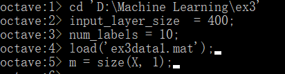
将数据集ex3data1.m和ex3weights.m文件复制到D:\Machine Learning\ex3文件目录下。
在ex3data1.mat中为您提供了一个数据集，其中包含5000个手写训练示例数字。ex3data1.mat中有5000个训练示例，其中每个训练示例都是数字的20像素×20像素灰度图像。每个像素由一个浮点数表示，该浮点数表示该位置的灰度强度。20×20像素网格被“展开”成一个400维的向量。在我们的数据矩阵X中，每一个训练例子都变成了一行。这给了我们一个5000×400的矩阵X，其中每一行都是手写数字图像的训练示例。训练集的第二部分是包含训练集标签的5000维向量y。在这里没有零索引，我们将数字0映射到值10。因此，“0”数字被标记为“10”，而数字“1”到“9”按其自然顺序标记为“1”到“9”。

1.2可视化数据

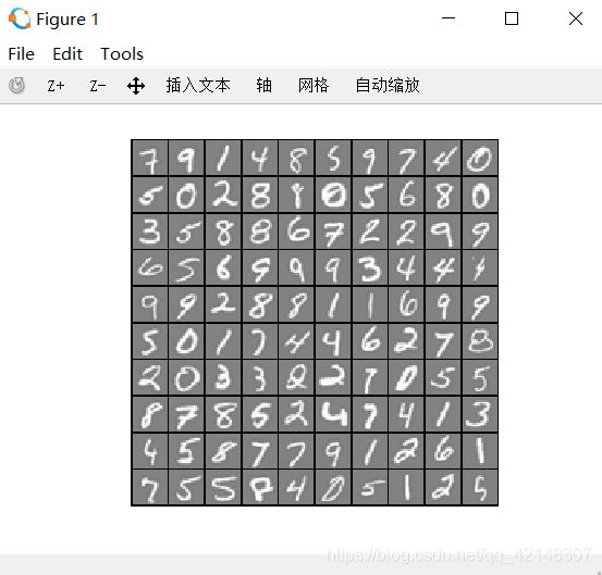
从X中随机选择100行，并将这些行传递给displayData函数。此函数将每行映射为20像素x 20像素的灰度图像，并将图像一起显示。在当前目录下建立displayData.m文件：

function [h, display_array] = displayData(X, example_width)
%返回两个参数，第一个就是绘制出的图形句柄；第二个就是100个处理后的案例图形的灰度强度矩阵
%第一个参数就是100个处理前的案例图形的灰度矩阵；第二个就是每个案例图形的显示宽度，用像素数表示
if ~exist('example_width', 'var') || isempty(example_width) 
 example_width = round(sqrt(size(X, 2)));
  %round计算离x最近的整数，如果没有设置案例图形的宽度，就设置为20
end
colormap(gray);
%将图形设置为灰度图型
[m n] = size(X);
example_height = (n / example_width);
%将每个案例图形的高度、宽度均这设置为20。
display_rows = floor(sqrt(m));
%当x为浮点数时，取小于x的最大整数，将每行放置10个案例
display_cols = ceil(m / display_rows);
%当x为浮点数时，取大于x的最小整数，将每列放置10个案例。
pad = 1;
%每个案例之间用一个像素的黑色线条进行填充，因为最终形成的
%display_array矩阵中填充地方的灰度强度为1，最高也就是为黑色
display_array = - ones(pad + display_rows * (example_height + pad), ...
                       pad + display_cols * (example_width + pad));
%生成像素矩阵，即多少行和多少列，每行每列代表一个像素。矩阵每个元素为1。
% 将X中案例图形的灰度强度矩阵复制到display_array矩阵中，中间进行略微调整。
curr_ex = 1;
for j = 1:display_rows
 for i = 1:display_cols
  if curr_ex > m, 
   break; 
  end
  max_val = max(abs(X(curr_ex, :)));
    %abs求绝对值，找出第一行中灰度强度最大的值，将每个案例处理后的
    %灰度强度矩阵的每个元素除以这个值，将灰度值归一化
  display_array(pad + (j - 1) * (example_height + pad) + (1:example_height), ...
                pad + (i - 1) * (example_width + pad) + (1:example_width)) = ...
      reshape(X(curr_ex, :), example_height, example_width) / max_val;
%reshape将每一行400列的矩阵转换成20*20的灰度强度矩阵，每个元素代表灰度强度，
%除以最大灰度强度，每个元素的灰度强度在-1到1之间；然后将每个20*20新生成的灰度强度矩阵
%赋值给display_array这个矩阵
  curr_ex = curr_ex + 1;
 end
 if curr_ex > m, 
  break; 
 end
end
h = imagesc(display_array, [-1 1]);
%画出灰度格图，第一个参数对应的是10*10个案例组成的灰度强度矩阵，每个元素代表不同的灰度强度。
%第二个参数代表灰度强度的范围是-1到1，-1就是白色，1就是黑色。
axis image off
%去掉坐标轴
drawnow;
%将去掉坐标轴的图形重新绘制出来
end

Octave中的操作：

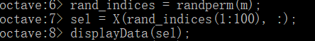
首先随机打乱m个数字序列，然后将前一百的数字序列对应的100行取出来形成矩阵X。然后绘制出相应的图片。绘制结果如图：

1.3向量化的逻辑回归

1.3.1成本函数的矢量化

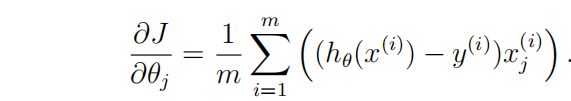
1.3.2梯度的矢量化

1.3.3矢量化正则化逻辑回归

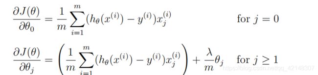
请注意，您不应该正则化θ0，它用于偏移项。A（：，2:end）将只返回从A的第2列到最后一列的元素。您可能需要使用元素级乘法运算（*）和写入此函数时的求和运算和

在当前目录下建立lrCostFunction.m文件，它的实现与正则化逻辑回归中costFunctionReg.m文件中实现的代码基本一致，只有最后要用元素级乘法运算：

function [J, grad] = lrCostFunction(theta, X, y, lambda)
m = length(y);
J = 0;
grad = zeros(size(theta));
J = sum(log(sigmoid(X * theta)) .* (-y) - log(1 - sigmoid(X * theta)) .* (1 - y)) / m;
J = J + lambda / 2 / m * (sum(theta.*theta) - theta(1)*theta(1));
grad = ((sigmoid(X * theta) - y)' * X / m)' ;
grad0 = grad(1);
grad  = grad + lambda / m * theta;
grad(1) = grad0;
grad = grad(:);
end

在当前目录下建立lsigmoid.m文件:

function g = sigmoid(z)
g = 1.0 ./ (1.0 + exp(-z));
end

打开Octave，将X_t、theta_t、y_t进行初始化，同时初始化λ。

1.4一对多分类

在这里没有零索引，我们将数字0映射到值10。因此，“0”数字被标记为“10”，而数字“1”到“9”按其自然顺序标记为“1”到“9”。
当训练类k∈{1，…，10}的分类器时，需要一个标签为y的m维向量，其中y_j∈0，1表示第j个训练实例是否属于类k（y_j=1），还是属于不同的类（y_j=0）

训练完一对多分类器之后，现在可以使用它来预测给定图像中包含的数字。对于每个输入，您应该使用经过训练的逻辑回归分类器计算它属于每个类的“概率”。您的一对多预测函数将选择对应的逻辑回归分类器输出最大概率的类，并返回类标签（1、2、…、或K）作为输入示例的预测。

在当前目录下建立oneVsAll.m文件，实现一对多分类器：

function [all_theta] = oneVsAll(X, y, num_labels, lambda)
%返回的是10*401的Θ矩阵；第三个参数是10，代表10类；第四个参数是λ
m = size(X, 1);
n = size(X, 2);
%m为5000，n为400
all_theta = zeros(num_labels, n + 1);
size(all_theta);
X = [ones(m, 1) X];
%给X增加常数项
initial_theta = zeros(n + 1, 1);
%all_theta的一列
options = optimset('GradObj', 'on', 'MaxIter', 50);
%迭代次数50次
for i=1:num_labels,
%共10列，组成all_theta矩阵
[theta] = fmincg (@(t)(lrCostFunction(t, X, (y == i), lambda)), ...
                 initial_theta, options);
%X是5000*401。y是5000*1,这里y矩阵是当y中元素等于i时为1，其余元素均为0。theta401*1
all_theta( i, : ) = theta';
end;

这里用到了 fmincg函数，fmincg的工作原理与fminunc类似，但在处理大量参数时更有效。具体实现我们利用别人提供的，仅展示代码，不加解释，会调用以及熟悉接口就行，在当前目录下建立fmincg.m文件：

function [X, fX, i] = fmincg(f, X, options, P1, P2, P3, P4, P5)
% Minimize a continuous differentialble multivariate function. Starting point
% is given by "X" (D by 1), and the function named in the string "f", must
% return a function value and a vector of partial derivatives. The Polack-
% Ribiere flavour of conjugate gradients is used to compute search directions,
% and a line search using quadratic and cubic polynomial approximations and the
% Wolfe-Powell stopping criteria is used together with the slope ratio method
% for guessing initial step sizes. Additionally a bunch of checks are made to
% make sure that exploration is taking place and that extrapolation will not
% be unboundedly large. The "length" gives the length of the run: if it is
% positive, it gives the maximum number of line searches, if negative its
% absolute gives the maximum allowed number of function evaluations. You can
% (optionally) give "length" a second component, which will indicate the
% reduction in function value to be expected in the first line-search (defaults
% to 1.0). The function returns when either its length is up, or if no further
% progress can be made (ie, we are at a minimum, or so close that due to
% numerical problems, we cannot get any closer). If the function terminates
% within a few iterations, it could be an indication that the function value
% and derivatives are not consistent (ie, there may be a bug in the
% implementation of your "f" function). The function returns the found
% solution "X", a vector of function values "fX" indicating the progress made
% and "i" the number of iterations (line searches or function evaluations,
% depending on the sign of "length") used.
%
% Usage: [X, fX, i] = fmincg(f, X, options, P1, P2, P3, P4, P5)
%
% See also: checkgrad 
%
% Copyright (C) 2001 and 2002 by Carl Edward Rasmussen. Date 2002-02-13
%
%
% (C) Copyright 1999, 2000 & 2001, Carl Edward Rasmussen
% 
% Permission is granted for anyone to copy, use, or modify these
% programs and accompanying documents for purposes of research or
% education, provided this copyright notice is retained, and note is
% made of any changes that have been made.
% 
% These programs and documents are distributed without any warranty,
% express or implied.  As the programs were written for research
% purposes only, they have not been tested to the degree that would be
% advisable in any important application.  All use of these programs is
% entirely at the user's own risk.
%
% [ml-class] Changes Made:
% 1) Function name and argument specifications
% 2) Output display
%
% Read options
if exist('options', 'var') && ~isempty(options) && isfield(options, 'MaxIter')
    length = options.MaxIter;
else
    length = 100;
end
RHO = 0.01;                            % a bunch of constants for line searches
SIG = 0.5;       % RHO and SIG are the constants in the Wolfe-Powell conditions
INT = 0.1;    % don't reevaluate within 0.1 of the limit of the current bracket
EXT = 3.0;                    % extrapolate maximum 3 times the current bracket
MAX = 20;                         % max 20 function evaluations per line search
RATIO = 100;                                      % maximum allowed slope ratio
argstr = ['feval(f, X'];                      % compose string used to call function
for i = 1:(nargin - 3)
  argstr = [argstr, ',P', int2str(i)];
end
argstr = [argstr, ')'];
if max(size(length)) == 2, red=length(2); length=length(1); else red=1; end
S=['Iteration '];
i = 0;                                            % zero the run length counter
ls_failed = 0;                             % no previous line search has failed
fX = [];
[f1 df1] = eval(argstr);                      % get function value and gradient
i = i + (length<0);                                            % count epochs?!
s = -df1;                                        % search direction is steepest
d1 = -s'*s;                                                 % this is the slope
z1 = red/(1-d1);                                  % initial step is red/(|s|+1)
while i < abs(length)                                      % while not finished
  i = i + (length>0);                                      % count iterations?!
  X0 = X; f0 = f1; df0 = df1;                   % make a copy of current values
  X = X + z1*s;                                             % begin line search
  [f2 df2] = eval(argstr);
  i = i + (length<0);                                          % count epochs?!
  d2 = df2'*s;
  f3 = f1; d3 = d1; z3 = -z1;             % initialize point 3 equal to point 1
  if length>0, M = MAX; else M = min(MAX, -length-i); end
  success = 0; limit = -1;                     % initialize quanteties
  while 1
    while ((f2 > f1+z1*RHO*d1) || (d2 > -SIG*d1)) && (M > 0) 
      limit = z1;                                         % tighten the bracket
      if f2 > f1
        z2 = z3 - (0.5*d3*z3*z3)/(d3*z3+f2-f3);                 % quadratic fit
      else
        A = 6*(f2-f3)/z3+3*(d2+d3);                                 % cubic fit
        B = 3*(f3-f2)-z3*(d3+2*d2);
        z2 = (sqrt(B*B-A*d2*z3*z3)-B)/A;       % numerical error possible - ok!
      end
      if isnan(z2) || isinf(z2)
        z2 = z3/2;                  % if we had a numerical problem then bisect
      end
      z2 = max(min(z2, INT*z3),(1-INT)*z3);  % don't accept too close to limits
      z1 = z1 + z2;                                           % update the step
      X = X + z2*s;
      [f2 df2] = eval(argstr);
      M = M - 1; i = i + (length<0);                           % count epochs?!
      d2 = df2'*s;
      z3 = z3-z2;                    % z3 is now relative to the location of z2
    end
    if f2 > f1+z1*RHO*d1 || d2 > -SIG*d1
      break;                                                % this is a failure
    elseif d2 > SIG*d1
      success = 1; break;                                             % success
    elseif M == 0
      break;                                                          % failure
    end
    A = 6*(f2-f3)/z3+3*(d2+d3);                      % make cubic extrapolation
    B = 3*(f3-f2)-z3*(d3+2*d2);
    z2 = -d2*z3*z3/(B+sqrt(B*B-A*d2*z3*z3));        % num. error possible - ok!
    if ~isreal(z2) || isnan(z2) || isinf(z2) || z2 < 0 % num prob or wrong sign?
      if limit < -0.5                               % if we have no upper limit
        z2 = z1 * (EXT-1);                 % the extrapolate the maximum amount
      else
        z2 = (limit-z1)/2;                                   % otherwise bisect
      end
    elseif (limit > -0.5) && (z2+z1 > limit)         % extraplation beyond max?
      z2 = (limit-z1)/2;                                               % bisect
    elseif (limit < -0.5) && (z2+z1 > z1*EXT)       % extrapolation beyond limit
      z2 = z1*(EXT-1.0);                           % set to extrapolation limit
    elseif z2 < -z3*INT
      z2 = -z3*INT;
    elseif (limit > -0.5) && (z2 < (limit-z1)*(1.0-INT))  % too close to limit?
      z2 = (limit-z1)*(1.0-INT);
    end
    f3 = f2; d3 = d2; z3 = -z2;                  % set point 3 equal to point 2
    z1 = z1 + z2; X = X + z2*s;                      % update current estimates
    [f2 df2] = eval(argstr);
    M = M - 1; i = i + (length<0);                             % count epochs?!
    d2 = df2'*s;
  end                                                      % end of line search
  if success                                         % if line search succeeded
    f1 = f2; fX = [fX' f1]';
    fprintf('%s %4i | Cost: %4.6e\r', S, i, f1);
    s = (df2'*df2-df1'*df2)/(df1'*df1)*s - df2;      % Polack-Ribiere direction
    tmp = df1; df1 = df2; df2 = tmp;                         % swap derivatives
    d2 = df1'*s;
    if d2 > 0                                      % new slope must be negative
      s = -df1;                              % otherwise use steepest direction
      d2 = -s'*s;    
    end
    z1 = z1 * min(RATIO, d1/(d2-realmin));          % slope ratio but max RATIO
    d1 = d2;
    ls_failed = 0;                              % this line search did not fail
  else
    X = X0; f1 = f0; df1 = df0;  % restore point from before failed line search
    if ls_failed || i > abs(length)          % line search failed twice in a row
      break;                             % or we ran out of time, so we give up
    end
    tmp = df1; df1 = df2; df2 = tmp;                         % swap derivatives
    s = -df1;                                                    % try steepest
    d1 = -s'*s;
    z1 = 1/(1-d1);                     
    ls_failed = 1;                                    % this line search failed
  end
  if exist('OCTAVE_VERSION')
    fflush(stdout);
  end
end
fprintf('\n');

在当前目录下建立predictOneVsAll.m文件预测给定图像中包含的数字，并且给出相应的概率（0到1之间）

function p = predictOneVsAll(all_theta, X)
m = size(X, 1);
num_labels = size(all_theta, 1);
p = zeros(size(X, 1), 1);
%p为5000*1
X = [ones(m, 1) X];
[a, p] = max( X * all_theta', [], 2);
% x为5000*401，all_theta为10*401,结果5000*10为每个个例为10个不同数字
%对应的概率（0至1），这里0对应第10列。max函数返回5000*10这个矩阵每一行的最大值
%a保存每一行最大值，也就是概率；p保存索引，也就是预测的数字。
end

打开Octave :

1. 设置λ，调用oneVsAll
2. 调用predictOneVsAll
   
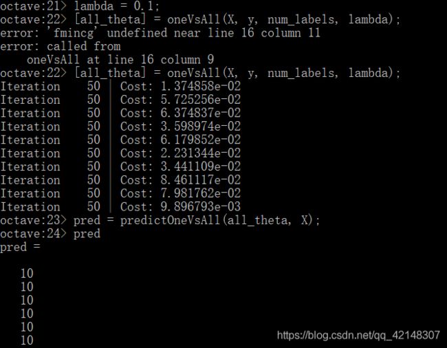
   预测成功的概率为95.060%

2、神经网络

您实现了多类逻辑回归来识别手写数字。然而，逻辑回归只是一个线性分类器，不能形成更复杂的假设。神经网络将能够代表形成非线性假设的复杂模型。本周，你们将使用我们已经训练过的神经网络的参数。您的目标是实现前馈传播算法，以使用我们的权重进行预测。在下周的练习中，您将编写用于学习神经网络参数的反向传播算法。

将ex3weights数据集复制到当前文件夹中，(Θ⁽¹⁾)Theta1是输入层映射到隐藏层的权重的矩阵；(Θ⁽²⁾)Theta2是隐藏层映射到输出层的权重的矩阵。输入层400+1个节点；隐藏层25+1个节点；输出层10个节点。

2.1前馈传播与预测

根据输入层输入的数据集数据，Theta1和Theta2预测出输出层的结果。因此首先得编写预测函数，之后，一个交互式序列将启动显示来自训练集的图像，一次一个，而控制台打印出所显示图像的预测标签。要停止图像序列，请按q。在当前目录下建立predict.m文件：

function p = predict(Theta1, Theta2, X)
%返回的是预测
m = size(X, 1);
num_labels = size(Theta2, 1);
size(X);
%5000*400
size(Theta1);
%25*401
size(Theta2);
%10*26
p = zeros(size(X, 1), 1);
%5000*1
X = [ones(m,1) X];
sec = sigmoid(X * Theta1');  
sec = [ones(m,1) sec];
%5000*26
fin = sigmoid(sec * Theta2');
%5000*10
[a, p] = max(fin, [], 2);
%保存每一行的最大值，以及返回相应的序号。
end

Octave中的操作：

1. 加载数据，对某些变量进行设置，随机抽出100个例，然后绘制出个例的图像。
2. 加载Theta数据集，对随机抽出的100个例进行预测，看预测成功的概率
3. 再一次打乱序号，一个交互式序列将启动显示来自训练集的图像，一次一个，而控制台打印出所显示图像的预测标签。要停止图像序列，请按q。mod是求余函数。
   
   
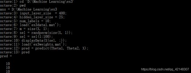
   预测成功的概率是97.520%
   
   
   
   
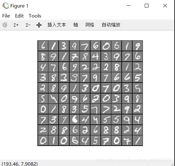
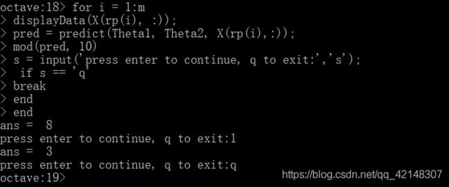
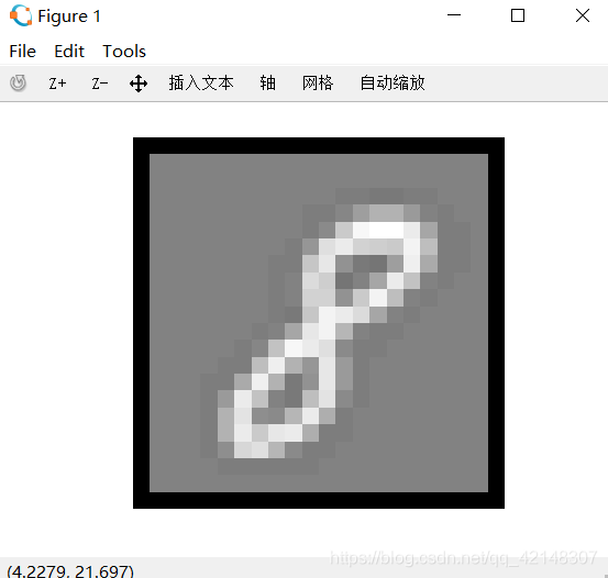
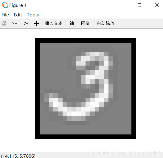
   图片所展示的8和3也都正确预测出来了。有意思的文字识别!