pytorch：词嵌入，词性判别，使用LSTM预测股票行情

文本数据处理

自然语言处理中，机器是无法直接理解人类语言的，因此就需要将语言数字化。就可以使用词向量，简单来说就是对字典 D 中所有词 w， 指定一个固定长度的实值向量

然后用pytorch的词嵌入模块吧语句用词向量表示，将这些词向量导入GRU 模型，这就是自然语言处理的基础也是核心。

>>> import jieba
>>> text = '阿巴阿巴阿巴阿巴\n狗头强行增加难度滑稽'
>>> words = list(jieba.cut(text))
Building prefix dict from the default dictionary ...
Dumping model to file cache C:\Users\ADMINI~1\AppData\Local\Temp\jieba.cache
Loading model cost 1.127 seconds.
Prefix dict has been built successfully.
>>> words
['阿巴', '阿巴', '阿巴', '阿巴', '\n', '狗头', '强行', '增加', '难度', '滑稽']
>>> stoplist = ['','\n']
>>> words = [i for i in words if i not in stoplist]          # 去掉一些终止词
>>> words
['阿巴', '阿巴', '阿巴', '阿巴', '狗头', '强行', '增加', '难度', '滑稽']

word_to_ix = {
      i: word for i, word in enumerate(set(words))}  # set 去重
# {0: '滑稽', 1: '狗头', 2: '强行', 3: '增加', 4: '阿巴', 5: '难度'}

from torch import nn
import torch
embeds = nn.Embedding(6, 8)    # 参数是词总数，生成的向量长度
lists=[]                     # 将离散变量转变为连续向量
for k,v in word_to_ix.items():
    tensor_value=torch.tensor(k)
    lists.append((embeds(tensor_value).data))
    
lists
[tensor([-0.5493, -1.2060, -0.9744, -0.2444,  0.0891,  1.0731, -0.4386, -0.5824]),
 tensor([ 0.1707,  0.5524,  1.3295, -0.1501, -0.0377, -0.9688, -0.1316, -0.0822]),
 tensor([-0.2302, -0.8453, -0.7160, -1.4149, -1.8610,  1.1420, -0.3238, -0.4046]),
 tensor([ 1.4589,  1.9889, -0.9287, -0.4668,  0.3158, -0.8721,  0.6879, -1.2364]),
 tensor([-2.2396,  0.2324,  0.2702, -1.2532,  0.4750,  0.9863, -0.5210,  0.0603]),
 tensor([ 0.9199,  0.7209, -1.2843, -0.9609, -0.7684,  0.5942,  0.0766,  0.1466])]

词嵌入

如果我们要把语句或文档让机器认识出，首先需要把这些语句或文档转成数字。上面产生词向量的任务就是词嵌入。将词转换为向量，最开始采用独热编码，再使用Bag_of_Worlds ，使用词频信息对对语句表示，后再就使用TF-IDF 根据词语再文本中分布情况表示，今年来随着神经网络的发展，分布式词语表达 word2Vec 对词语进行连续的多维向量表示。

分布式表示，可以克服独热编码的维度灾难，和不能体现词与词之间的关系的缺点。可以通过计数向量之间的距离（欧氏距离）来体现词与词的相似性。训练这种向量的方法有很多，比如Word2Vec 等，这是一个词向量计算工具，同时也是一套生成词向量的算法方案。这个算法的背后是3 层神经网络，生成的词向量再很多任务中都可以作为深度学习算法的输入，所以说Word2Vec 技术是深度学习再NLP 领域的基础。

Word2Vec 原理

模型的两种模式，CBOW 模型（对于每一个词汇，使用周围的词汇来预测当前词汇生成的概率）和 SkipGram 模型（对于每一个词汇，使用该词汇本身来预测生成其他词汇的概率）。根据上下文生成目标值使用CBOW模型，根据目标值生成上下文使用Skip-Gram模型。
两个方法的 限制就是对于相同的输入，输出的每个词汇的概率之和为1。

CBOW模型

cbow模型包括三层，输入出，映射层，输出层 。 目标词w(t) ，再其已知的上下文 w(t-2), w(t-1), w(t+1), w(t+2) 的前提下进行预测，即 p(w| context(w) ):

$L=\sum \log p(w|context(w))$

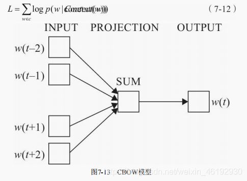
CBOW 模型训练就是根据某个词前后若干词来预测该词，可以看成多分类。最简单的就是直接使用softmax 来分别计算每个词对应的归一化概率，对于几十万词汇量的场景中使用softmax 计算量太大，需要使用一种二分类组合形式的 分层的 Softmax ，即输出层为一个二叉树

Skip-Gram模型

同样包含三层，输入层，映射层，输出层。这个与CBOW 模型相反，使用已知词来预测其上下文，目标函数为：

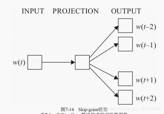
比如，对于一个句子： the quick brown fox jumped over the lazy dog 。对这些单词和他们的上下文环境生成数据集，这里使用大小为1 的窗口，也就是选择目标单词的左右一个单词作为上下文与输入词进行组合：

使用pytorch实现词性判别

一个单词，具体表现为那种词性，要根据这个词的上文，这就很适合使用循环神经网络，LSTM OR GRU 具有记忆功能

步骤

1. 构架词向量，假如有两个句子，作为训练数据这两个句子的每个单词的词性已知，输入前需要把每个单词量化得到序列，然后输入LSTM模型。（nn.Embedding)
2. 构建网络，可以构建一个只有3层的网络，第一层位词嵌入，第二层位LSTM 层，最后一次用来词性的分类全连接。

word_to_ix = {
     } # 单词的索引字典
for sent, tags in training_data:
    for word in sent:
        if word not in word_to_ix:
            word_to_ix[word] = len(word_to_ix)
print(word_to_ix)
#两句话,共有9个不同单词
#{'The': 0, 'cat': 1, 'ate': 2, 'the': 3, 'fish': 4, 'They': 5, 'read': 6, 'that': 7, 'book': 8}
{
     'The': 0, 'cat': 1, 'ate': 2, 'the': 3, 'fish': 4, 'They': 5, 'read': 6, 'that': 7, 'book': 8}


tag_to_ix = {
     "DET": 0, "NN": 1, "V": 2} # 词性索引字典


# 构建网络
import torch.nn as nn
import torch.nn.functional as F
import torch
class LSTMTagger(nn.Module):
    def __init__(self,embedding_dim,hidden_dim,vocab_size,tagset_size):
        super(LSTMTagger,self).__init__()
        self.hidden_dim = hidden_dim
        self.word_embeddings = nn.Embedding(vocab_size,embedding_dim) # 词总数，词向量的长度
        self.lstm = nn.LSTM(embedding_dim,hidden_dim)
        self.hidden2tag = nn.Linear(hidden_dim,tagset_size)
        self.hidden = self.init_hidden()

    def init_hidden(self): # LSTM有两个隐藏状态
        return (torch.zeros(1,1,self.hidden_dim),torch.zeros(1,1,self.hidden_dim))

    def forward(self,sentence):
        # 获得词嵌入矩阵
        embeds = self.word_embeddings(sentence)
        # 送入LSTM ，注意修改形状，隐藏层维度也要匹配
        # lstm_out (seq_len，batch，num_directions * hidden_​​size)
        lstm_out,self.hidden = self.lstm(embeds.view(len(sentence),1,-1),self.hidden)
        # 一个全连接，对应到标签
        tag_space = self.hidden2tag(lstm_out.view(len(sentence),-1))
        # 计算每个单词属于各个词性的概率，这里返回的是对数的softmax结果 
        tag_scores = F.log_softmax(tag_space,dim=1)
        return tag_scores

# 将数据转换为LongTensor 的格式
def prepare_sequence(seq,to_ix):
    idx = [to_ix[w] for w in seq]
    tensor = torch.LongTensor(idx)
    return tensor


# 训练网络
EMBEDDING_DIM=10   # 词向量的长度
HIDDEN_DIM=3       #这里等于词性个数
model = LSTMTagger(EMBEDDING_DIM, HIDDEN_DIM, len(word_to_ix), len(tag_to_ix)) # 单词和词性标签的字典
loss_function = nn.NLLLoss()
optimizer = torch.optim.SGD(model.parameters(), lr=0.1)

# PS：vscode的jupyter notebook中 L 可以显示行号


# 将数据转换为LongTensor 的格式，并得到字典中的索引
def prepare_sequence(seq,to_ix):
    idx = [to_ix[w] for w in seq]
    tensor = torch.LongTensor(idx)


inputs = prepare_sequence(training_data[0][0], word_to_ix)
tag_scores = model(inputs)
print(training_data[0][0])
print(inputs)   # 对应的单词字典的索引
print(tag_scores)  # 得分
print(torch.max(tag_scores,1))   # 可以看到效果很不好。。
>>>
['The', 'cat', 'ate', 'the', 'fish']
tensor([0, 1, 2, 3, 4])
tensor([[-1.4884, -1.1565, -0.7772],
        [-1.4330, -1.2307, -0.7565],
        [-1.3792, -1.2462, -0.7752],
        [-1.3717, -1.2958, -0.7494],
        [-1.4788, -1.2665, -0.7128]], grad_fn=<LogSoftmaxBackward>)
torch.return_types.max(
values=tensor([-0.7772, -0.7565, -0.7752, -0.7494, -0.7128], grad_fn=<MaxBackward0>),
indices=tensor([2, 2, 2, 2, 2]))


for epoch in range(400): # 训练400次，加大精度
    for sentence, tags in training_data:
        # 清除网络先前的梯度值
        model.zero_grad()
        # 重新初始化隐藏层数据
        model.hidden = model.init_hidden()
        # 按网络要求的格式处理输入数据和真实标签数据
        sentence_in = prepare_sequence(sentence, word_to_ix)
        targets = prepare_sequence(tags, tag_to_ix)
        # 实例化模型
        tag_scores = model(sentence_in)
        # 计算损失,反向传递梯度及更新模型参数
        loss = loss_function(tag_scores, targets)
        loss.backward()
        optimizer.step()
# 查看模型训练的结果
inputs = prepare_sequence(training_data[0][0], word_to_ix)
tag_scores = model(inputs)
print(training_data[0][0])
print(tag_scores)
print(torch.max(tag_scores,1))   # 精度为100 %
>>>
['The', 'cat', 'ate', 'the', 'fish']
tensor([[-0.3022, -1.8708, -2.2367],
        [-6.6132, -0.0103, -4.7179],
        [-3.7927, -2.9967, -0.0752],
        [-0.0261, -5.7446, -3.7911],
        [-6.2870, -0.0074, -5.1993]], grad_fn=<LogSoftmaxBackward>)
torch.return_types.max(
values=tensor([-0.3022, -0.0103, -0.0752, -0.0261, -0.0074], grad_fn=<MaxBackward0>),
indices=tensor([0, 1, 2, 0, 1]))



test_inputs = prepare_sequence(testing_data[0], word_to_ix)
tag_scores01 = model(test_inputs)
print(testing_data[0])
print(test_inputs)
print(tag_scores01)
print(torch.max(tag_scores01,1))   # 使用测试的数据精度也为100%
>>>
['They', 'ate', 'the', 'fish']
tensor([5, 2, 3, 4])
tensor([[-6.4221e+00, -4.1696e-03, -5.9773e+00],
        [-3.8124e+00, -2.9920e+00, -7.5030e-02],
        [-2.6181e-02, -5.7439e+00, -3.7881e+00],
        [-6.2861e+00, -7.4140e-03, -5.1986e+00]], grad_fn=<LogSoftmaxBackward>)
torch.return_types.max(
values=tensor([-0.0042, -0.0750, -0.0262, -0.0074], grad_fn=<MaxBackward0>),
indices=tensor([1, 2, 0, 1]))

用LSTM预测股票行情

import tushare as ts
import matplotlib.pyplot as plt
import numpy as np
cons = ts.get_apis()  # 建立链接
#获取沪深指数(000300)的信息,包括交易日期(datetime)、开盘价(open)、收盘价(close),
#最高价(high)、最低价(low)、成交量(vol)、成交金额(amount)、涨跌幅(p_change)
df = ts.bar('000300', conn=cons, asset='INDEX', start_date='2010-01-01', end_date='')
#删除有null值的行
df = df.dropna()
#把df保存到当前目录下的sh300.csv文件中,以便后续使用
df.to_csv('sh300.csv')

df.columns
Index(['code', 'open', 'close', 'high', 'low', 'vol', 'amount', 'p_change'], dtype='object')

df_index = df.index
df_index = np.array(df_index)
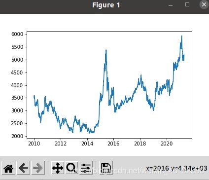
df_all = df['high']
df_all = np.array(df_all.tolist())
plt.plot(df_index,df_all)

# PS: jupyter 中切换matplotlib的后端 %matplotlib inline/auto  内部/外部显示
# sudo apt install python3-tk   # 下载tkinter

import pandas as pd
import matplotlib.pyplot as plt
import datetime
import torch
import torch.nn as nn
import numpy as np
from torch.utils.data import Dataset, DataLoader
import torchvision
import torchvision.transforms as transforms

# 数据预处理
n = 30
LR = 0.001
EPOCH = 200
batch_size=20
train_end =-500

device = torch.device('cuda' if torch.cuda.is_available() else 'cpu')

#通过一个序列来生成一个31*(count(*)-train_end)矩阵(用于处理时序的数据)
#其中最后一列为标签数据。就是把当天的前n天作为参数,当天的数据作为label，理解不了可以看看最后返回的数据
def generate_data_by_n_days(series, n, index=False):
    if len(series) <= n:
        raise Exception("The Length of series is %d, while affect by (n=%d)." % (len(series), n))
    df = pd.DataFrame()
    for i in range(n):
    # 隔一天拼出一列    2218*30
        df['c%d' % i] = series.tolist()[i:-(n - i)]
    df['y'] = series.tolist()[n:]
    if index:
        df.index = series.index[n:]
    return df   # shape 2218 rows × 31 columns

# 参数n与上相同。train_end表示的是后面多少个数据作为测试集。
def readData(column='high', n=30, all_too=True, index=False, train_end=-500):
    df = pd.read_csv("sh300.csv", index_col=0)
    #以日期为索引
    df.index = list(map(lambda x: datetime.datetime.strptime(x, "%Y-%m-%d"), df.index))
    #获取每天的最高价
    df_column = df[column].copy()
    #拆分为训练集和测试集
    df_column_train, df_column_test = df_column[:train_end], df_column[train_end - n:] 
    # 测试集多加了三十天
    # df_column_train.shape, df_column_test.shape  ((2248,), (530,))
    #生成训练数据
    df_generate_train = generate_data_by_n_days(df_column_train, n, index=index) 
    if all_too:
        return df_generate_train, df_column, df.index.tolist()
    return df_generate_train

看看最后的数据就好理解了，，，Typora真好使啊。。这些数据就可以用来训练LSTM，以前三十天为参数，最后一天为标签

	c0	c1	c2	c3	c4	c5	c6	c7	c8	c9	…	c21	c22	c23	c24	c25	c26	c27	c28	c29	y
0	5181.11	5149.98	5119.22	5110.56	5119.86	5088.21	4979.17	4969.91	4987.12	4994.54	…	4950.76	5024.33	5064.02	5071.34	5089.92	5160.46	5123.55	5084.31	5120.88	5153.67
1	5149.98	5119.22	5110.56	5119.86	5088.21	4979.17	4969.91	4987.12	4994.54	5045.60	…	5024.33	5064.02	5071.34	5089.92	5160.46	5123.55	5084.31	5120.88	5153.67	5138.41
2	5119.22	5110.56	5119.86	5088.21	4979.17	4969.91	4987.12	4994.54	5045.60	5100.04	…	5064.02	5071.34	5089.92	5160.46	5123.55	5084.31	5120.88	5153.67	5138.41	5055.28
3	5110.56	5119.86	5088.21	4979.17	4969.91	4987.12	4994.54	5045.60	5100.04	5129.13	…	5071.34	5089.92	5160.46	5123.55	5084.31	5120.88	5153.67	5138.41	5055.28	5094.31
4	5119.86	5088.21	4979.17	4969.91	4987.12	4994.54	5045.60	5100.04	5129.13	5141.66	…	5089.92	5160.46	5123.55	5084.31	5120.88	5153.67	5138.41	5055.28	5094.31	5326.26
…	…	…	…	…	…	…	…	…	…	…	…	…	…	…	…	…	…	…	…	…	…
2213	2622.66	2631.05	2624.32	2618.25	2705.75	2681.33	2666.43	2664.41	2645.95	2628.59	…	2574.75	2558.35	2559.35	2562.07	2533.26	2553.45	2560.03	2546.03	2534.16	2489.03
2214	2631.05	2624.32	2618.25	2705.75	2681.33	2666.43	2664.41	2645.95	2628.59	2657.96	…	2558.35	2559.35	2562.07	2533.26	2553.45	2560.03	2546.03	2534.16	2489.03	2520.76
2215	2624.32	2618.25	2705.75	2681.33	2666.43	2664.41	2645.95	2628.59	2657.96	2694.61	…	2559.35	2562.07	2533.26	2553.45	2560.03	2546.03	2534.16	2489.03	2520.76	2514.65
2216	2618.25	2705.75	2681.33	2666.43	2664.41	2645.95	2628.59	2657.96	2694.61	2679.93	…	2562.07	2533.26	2553.45	2560.03	2546.03	2534.16	2489.03	2520.76	2514.65	2486.24
2217	2705.75	2681.33	2666.43	2664.41	2645.95	2628.59	2657.96	2694.61	2679.93	2647.79	…	2533.26	2553.45	2560.03	2546.03	2534.16	2489.03	2520.76	2514.65	2486.24	2481.66

2218 rows × 31 columns

# 获取训练数据、原始数据、索引等信息
df, df_all, df_index = readData('high', n=n, train_end=train_end)
#可视化最高价，，，，效果同上。。。。
df_all = np.array(df_all.tolist())
plt.plot(df_index, df_all, label='real-data')
plt.legend(loc='upper right')

class mytrainset(Dataset):
    def __init__(self, data):        
        self.data, self.label = data[:, :-1].float(), data[:, -1].float()
             
    def __getitem__(self, index):
        return self.data[index], self.label[index]

    def __len__(self):
        return len(self.data)


class RNN(nn.Module):
    def __init__(self,input_size):
        super(RNN,self).__init__()
        self.rnn = nn.LSTM(
            input_size = input_size,
            hidden_size = 64,
            num_layers = 1,
            batch_first = True
            # 输入和输出张量按（batch，seq，feature)提供
        )
        self.out = nn.Sequential(nn.Linear(64,1))
    def forward(self,x):
        r_out,(h_n,h_c) = self.rnn(x,None)
        # print('r_out.shape = ',r_out.shape)
        out = self.out(r_out)
        return out


# 对数据进行预处理,规范化及转换为Tensor
df_numpy = np.array(df)
df_numpy_mean = np.mean(df_numpy)
df_numpy_std = np.std(df_numpy)
df_numpy = (df_numpy - df_numpy_mean) / df_numpy_std  
df_tensor = torch.Tensor(df_numpy)
trainset = mytrainset(df_tensor)
trainloader = DataLoader(trainset, batch_size=batch_size, shuffle=False)


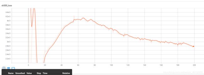
#记录损失值，并用tensorboardx在web上展示
from tensorboardX import SummaryWriter
os.environ['CUDA_VISIBLE_DEVICES'] = '0'
writer = SummaryWriter(log_dir='logs')

rnn = RNN(n).to(device)
optimizer = torch.optim.Adam(rnn.parameters(), lr=LR)  
loss_func = nn.MSELoss()

for step in range(EPOCH):
    for tx, ty in trainloader:
        tx=tx.to(device)   # (30,20)
        ty=ty.to(device)   # (20)
        #在第1个维度上添加一个维度为1的维度，形状变为[batch,seq_len,input_size]
        output = rnn(torch.unsqueeze(tx, dim=1)).to(device)
        loss = loss_func(torch.squeeze(output), ty)
        optimizer.zero_grad()  
        loss.backward()  
        optimizer.step()
    writer.add_scalar('sh300_loss', loss, step)  

generate_data_train = []
generate_data_test = []

test_index = len(df_all) + train_end   # 最高点的那些数据

df_all_normal = (df_all - df_numpy_mean) / df_numpy_std
df_all_normal_tensor = torch.Tensor(df_all_normal)
for i in range(n, len(df_all)):
    x = df_all_normal_tensor[i - n:i].to(device)  # 30个一组
    #rnn的输入必须是3维，故需添加两个1维的维度，最后成为[1,1,input_size]
    x = torch.unsqueeze(torch.unsqueeze(x, dim=0), dim=0)
    
    y = rnn(x).to(device)
    if i < test_index:
        generate_data_train.append(torch.squeeze(y).detach().cpu().numpy() * df_numpy_std + df_numpy_mean)
    else:
        generate_data_test.append(torch.squeeze(y).detach().cpu().numpy() * df_numpy_std + df_numpy_mean)

plt.plot(df_index[n:train_end], generate_data_train, label='generate_train')
plt.plot(df_index[train_end:], generate_data_test, label='generate_test')
plt.plot(df_index[train_end:], df_all[train_end:], label='real-data')
plt.legend()
plt.show()

注意数据的时间是反序的，所以test数据集在前面。可以看出预测出的数据和真实数据很相似。

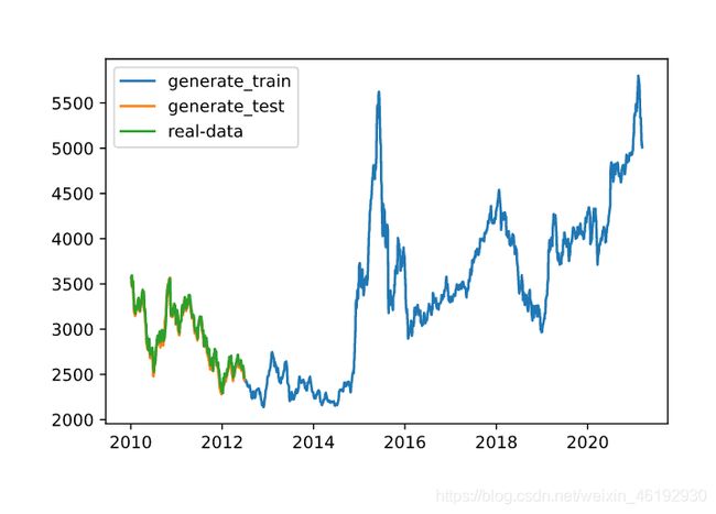
放大来看的话还是有差距的。。。。。不过效果挺好的。。。。

plt.clf()
plt.plot(df_index[train_end:-500], df_all[train_end:-500], label='real-data')
plt.plot(df_index[train_end:-500], generate_data_test[-600:-500], label='generate_test')
plt.legend()
plt.show()