- LangChain中的向量数据库接口-Weaviate
洪城叮当
langchain数据库经验分享笔记交互人工智能知识图谱
文章目录前言一、原型定义二、代码解析1、add_texts方法1.1、应用样例2、from_texts方法2.1、应用样例3、similarity_search方法3.1、应用样例三、项目应用1、安装依赖2、引入依赖3、创建对象4、添加数据5、查询数据总结前言 Weaviate是一个开源的向量数据库,支持存储来自各类机器学习模型的数据对象和向量嵌入,并能无缝扩展至数十亿数据对象。它提供存储文档嵌
- Python的科学计算库NumPy(一)
linlin_1998
pythonnumpy开发语言
NumPy(NumericalPython)是Python中最基础、最重要的科学计算库之一,提供了高性能的多维数组(ndarray)对象和大量数学函数,是许多数据科学、机器学习库(如Pandas、SciPy、TensorFlow等)的基础依赖。1.创建一个numpy里面的一维数组importnumpyasnp###通过array方法创建一个ndarrayarray1=np.array([1,2,3
- 微算法科技的前沿探索:量子机器学习算法在视觉任务中的革新应用
MicroTech2025
量子计算算法
在信息技术飞速发展的今天,计算机视觉作为人工智能领域的重要分支,正逐步渗透到我们生活的方方面面。从自动驾驶到人脸识别,从医疗影像分析到安防监控,计算机视觉技术展现了巨大的应用潜力。然而,随着视觉任务复杂度的不断提升,传统机器学习算法在处理大规模、高维度数据时遇到了计算瓶颈。在此背景下,量子计算作为一种颠覆性的计算模式,以其独特的并行处理能力和指数级增长的计算空间,为解决这一难题提供了新的思路。微算
- 在mac m1基于llama.cpp运行deepseek
lama.cpp是一个高效的机器学习推理库,目标是在各种硬件上实现LLM推断,保持最小设置和最先进性能。llama.cpp支持1.5位、2位、3位、4位、5位、6位和8位整数量化,通过ARMNEON、Accelerate和Metal支持Apple芯片,使得在MACM1处理器上运行Deepseek大模型成为可能。1下载llama.cppgitclonehttps://github.com/ggerg
- 【机器学习笔记Ⅰ】9 特征缩放
巴伦是只猫
机器学习机器学习笔记人工智能
特征缩放(FeatureScaling)详解特征缩放是机器学习数据预处理的关键步骤,旨在将不同特征的数值范围统一到相近的尺度,从而加速模型训练、提升性能并避免某些特征主导模型。1.为什么需要特征缩放?(1)问题背景量纲不一致:例如:特征1:年龄(范围0-100)特征2:收入(范围0-1,000,000)梯度下降的困境:量纲大的特征(如收入)会导致梯度更新方向偏离最优路径,收敛缓慢。量纲小的特征(如
- 深度学习实战-使用TensorFlow与Keras构建智能模型
程序员Gloria
Python超入门TensorFlowpython
深度学习实战-使用TensorFlow与Keras构建智能模型深度学习已经成为现代人工智能的重要组成部分,而Python则是实现深度学习的主要编程语言之一。本文将探讨如何使用TensorFlow和Keras构建深度学习模型,包括必要的代码实例和详细的解析。1.深度学习简介深度学习是机器学习的一个分支,使用多层神经网络来学习和表示数据中的复杂模式。其广泛应用于图像识别、自然语言处理、推荐系统等领域。
- 【大模型与机器学习解惑】什么是A/B测试,为何进行A/B测试?
以下内容将围绕机器学习中的A/B测试展开,从概念与背景到实施细节、示例代码、优化思路和未来建议,并在最后给出一个整体的“输出目录”供参考。目录什么是机器学习的A/B测试为何要进行A/B测试A/B测试的实施流程示例代码与详细解释优化方向与未来建议结语1.什么是机器学习的A/B测试A/B测试(也常被称作对照试验、SplitTest)最早多用于互联网产品的功能或界面迭代中,指的是将用户或样本随机分为两组
- 详解LLMOps,将DevOps用于大语言模型开发
大家好,在机器学习领域,随着技术的不断发展,将大型语言模型(LLMs)集成到商业产品中已成为一种趋势,同时也带来了许多挑战。为了有效应对这些挑战,数据科学家们转向了一种新型的DevOps实践LLM-OPS,专为大型语言模型的开发和维护而设计。本文将介绍LLM-OPS的核心思想,并分析这一策略如何帮助数据科学家更高效地运用DevOps的优秀实践,从而在语言模型的开发和部署过程中,提升工作效率和成果的
- 搜广推校招面经九十一
美团机器学习/数据挖掘算法工程师_二面一、介绍一下ESMM模型,是否有进行过函数推导传统的转化率建模方式:只用发生点击(click=1)的样本来训练CVR模型。CVR定义如下:CVR=P(y=1∣x,z=1)CVR=P(y=1|x,z=1)CVR=P(y=1∣x,z=1)y=1表示用户发生了转化(如购买)z=1表示用户点击了广告这样做的问题:样本选择偏差(SampleSelectionBias,S
- python 计算生态概览的概述
文章目录前言python计算生态库的介绍1.网络爬虫2.数据分析3.文本处理4.数据可视化5.机器学习6.图形用户界面7.游戏开发8.网络应用开发前言python计算生态概览的解释Python计算生态概览是对Python作为一门强大而广泛使用的编程语言所拥有的庞大软件集合的整体描述和概述。这个生态体系不仅包含了Python的标准库(stdlib),即随Python解释器安装的基本模块,还涵盖了极其
- Google机器学习实践指南(模型预测偏差)
AI_Auto
人工智能机器学习人工智能
Google机器学习(31)-模型预测偏差预测偏差:模型为何总是"猜不准"的真相揭秘你的模型预测准确率高达95%,却总是与实际情况差那么一点点?这可能是预测偏差在作祟!本文将带你深入探索这个被忽视的模型"隐形杀手"。一、什么是预测偏差?一个生活化案例想象一下,你网购了一个智能体重秤,连续一周称重显示都是60kg。但你去健身房用专业设备测量,实际是62kg。这种系统性的测量偏差,就是预测偏差在现实中
- 【机器学习|学习笔记】用 Python 结合 graphviz 生成 ID3、C4.5、CART 三种决策树的结构示意图。
【机器学习|学习笔记】用Python结合graphviz生成ID3、C4.5、CART三种决策树的结构示意图【机器学习|学习笔记】用Python结合graphviz生成ID3、C4.5、CART三种决策树的结构示意图文章目录【机器学习|学习笔记】用Python结合graphviz生成ID3、C4.5、CART三种决策树的结构示意图用Python结合graphviz生成ID3、C4.5、CART三种
- 智能产品经理的核心能力
AI天才研究院
AgenticAI实战AI人工智能与大数据AI大模型企业级应用开发实战计算科学神经计算深度学习神经网络大数据人工智能大型语言模型AIAGILLMJavaPython架构设计AgentRPA
智能产品经理的核心能力1.背景介绍在当今快节奏的数字时代,产品经理扮演着至关重要的角色,他们负责确保产品满足用户需求,实现商业目标,并保持竞争优势。随着人工智能(AI)和机器学习(ML)技术的不断发展,智能产品经理的概念应运而生。智能产品经理需要将传统的产品管理技能与新兴技术相结合,以创建具有创新性和智能化的产品体验。智能产品不仅需要满足功能需求,还需要提供个性化、智能化和无缝的用户体验。这对产品
- 使用Python进行机器学习入门指南
软考和人工智能学堂
Python开发经验python机器学习开发语言
使用Python进行机器学习入门指南机器学习(MachineLearning)是人工智能(ArtificialIntelligence,AI)的一个重要分支,旨在通过算法和统计模型,使计算机系统能够自动从数据中学习和改进。Python作为机器学习领域的主流编程语言,提供了丰富的库和工具来实现各种机器学习任务。本文将介绍如何使用Python进行机器学习,包括基本概念、常用库以及一个实战项目示例。目录
- 【亲测免费】 CatBoost 教程项目使用指南
CatBoost教程项目使用指南tutorials项目地址:https://gitcode.com/gh_mirrors/tutorials1/tutorials1.项目介绍CatBoost是一个高效、灵活且易于使用的梯度提升库,特别适用于处理分类特征。它由Yandex开发,广泛应用于机器学习和数据科学领域。CatBoost提供了丰富的功能,包括自动处理分类特征、支持GPU训练、内置的交叉验证和模
- Python自动化机器学习平台库之mindsdb使用详解
概要MindsDB是一个开源的自动化机器学习平台,它通过SQL接口简化了机器学习模型的创建、训练和预测过程。该库的核心理念是将机器学习功能直接集成到数据库中,让开发者无需深入了解复杂的机器学习算法,就能够快速构建和部署预测模型。MindsDB支持多种数据源连接,包括MySQL、PostgreSQL、MongoDB等主流数据库,同时提供了丰富的PythonAPI接口,使得数据科学家和开发者能够在熟悉
- 堡垒机操作行为异常检测的机器学习算法应用
一、传统检测模式的困境与机器学习的破局价值在数字化转型浪潮中,堡垒机作为运维安全的核心防线,面临着操作行为复杂度激增与检测能力滞后的双重挑战。传统检测手段主要依赖静态规则库与统计模型,存在三大致命缺陷:规则固化与误报泛滥:某金融机构曾因规则库未及时更新,导致运维人员正常批量操作被误判为“暴力破解”,单日误报量超2000次,消耗安全团队60%的精力。动态行为适应性弱:微服务架构下,运维人员访问路径呈
- 最全 自动驾驶数据集 (11/4号已更新)
数据猎手小k
自动驾驶人工智能机器学习
自动驾驶是一个快速发展的行业,它融合了人工智能、机器学习、传感器技术、高精度地图和先进的计算平台等多种技术。技术方面,自动驾驶汽车依赖于先进的传感器、如激光雷达、摄像头、毫米波雷达等,以及强大的计算平台来处理大量数据,自动驾驶数据集是训练和验证自动驾驶系统的关键资源,它提供了丰富的场景和条件,使算法能够学习和适应复杂的真实世界驾驶环境。一、研究背景自动驾驶技术的发展需要大量的数据来训练和优化算法,
- 机器学习深度学习驱动在光子学设计中的应用与未来【专题培训会议邀您共探科技前沿】
软研科技
信息与通信信号处理量子计算人工智能
一、背景介绍在智能科技飞速发展的今天,光子学设计与智能算法的结合正成为科研创新的热点。深度学习、机器学习等算法在光子器件的逆向设计、超构表面材料设计、光学神经网络构建等方面展现出巨大潜力。二、会议亮点由北京软研国际信息技术研究院主办的“智能算法驱动的光子学设计与应用”专题培训会议,将深入探讨以下核心内容:光子器件的逆向设计:利用深度学习优化多参数光子器件设计。超构表面与超材料设计:智能算法在新型光
- 机器学习与光子学的融合正重塑光学器件设计范式
m0_75133639
光电智能电视二维材料电子半导体人工智能顶刊nature
Nature/Science最新研究表明,该交叉领域聚焦六大前沿方向:光子器件逆向设计、超构材料智能优化、光子神经网络加速器、非线性光学芯片开发、多任务协同优化及光谱智能预测。系统掌握该领域需构建四维知识体系:1、基础融合——从空间/集成光学系统切入,解析机器学习赋能光学的理论必然性,涵盖光学神经网络构建原理2、逆向设计革命——通过AnsysOptics实战,掌握FDTD算法与粒子群/拓扑优化技术
- AI模型训练新范式:基于同态加密的隐私保护方案
AIGC应用创新大全
人工智能同态加密区块链ai
AI模型训练新范式:基于同态加密的隐私保护方案技术解析关键词同态加密(HomomorphicEncryption)、隐私保护机器学习(PPML)、全同态加密(FHE)、安全多方计算(MPC)、加密数据训练摘要本报告系统解析基于同态加密的AI模型训练新范式,覆盖从理论基础到工程实践的全生命周期。首先通过第一性原理推导同态加密的数学本质,对比传统隐私保护技术的局限性;其次构建“加密-训练-解密”全流程
- 量子机器学习入门:从理论到实践
量子机器学习入门:从理论基石到实践路径元数据框架标题量子机器学习入门:从理论基石到实践路径——连接量子计算与人工智能的未来桥梁关键词量子计算;机器学习;量子算法;量子神经网络;Qiskit;PennyLane;量子变分算法摘要量子机器学习(QuantumMachineLearning,QML)是量子计算与机器学习的交叉领域,通过量子计算的叠加态、纠缠和并行性解决传统机器学习的计算瓶颈(如高维数据处
- 全球人工智能与机器学习大会PPT
a flying bird
论文解读和大咖技术号记录人工智能
大会演讲PPT合集https://ppt.infoq.cn/list/93PPT分享|ppt|人工智能|aicon|infoq|机器学习PPT分享,前段时间的AICon北京站2021全球人工智能与机器学习大会(https://aicon.infoq.cn/2021/beijing),汇集了很多业界大佬,工业界多个方向的从业人员分享了他们在实际业……https://xw.qq.com/cmsid/2
- 人工智能基础知识PPT课件
智慧化智能化数字化方案
方案解读馆人工智能入门人工智能学习人工智能课件人工智能PPT
人工智能基础知识定义与概念:人工智能是研究、开发用于模拟、延伸和扩展人类智能行为的综合性科学,其目的是让计算机系统具备执行人类智能任务的能力。涉及计算机科学、数学等多学科,研究对象是让系统具备智能,智能包括认知、适应和自主能力等维度。学派与方法学派:有符号主义、联结主义、行为主义等学派,分别从不同角度研究人工智能。方法:包括基于知识、学习和仿生的方法,如专家系统、机器学习、深度学习等。分类与发展分
- 数据挖掘:从理论到实践的深度探索
代码老y
数据挖掘人工智能
在当今数字化时代,数据已经成为企业决策的重要依据。数据挖掘作为一门从大量数据中提取有价值信息的技术,已经广泛应用于各个领域,如金融、医疗、零售、互联网等。本文将深入探讨数据挖掘的基本概念、主要技术和实际应用案例,帮助读者更好地理解数据挖掘的价值和应用。一、数据挖掘的基本概念(一)数据挖掘的定义数据挖掘(DataMining)是从大量数据中提取有用信息的过程。它结合了统计学、机器学习、数据库技术和人
- 开发智能化的企业并购风险评估模型
开发智能化的企业并购风险评估模型关键词:企业并购、风险评估、人工智能、机器学习、深度学习、数学建模摘要:本文详细探讨了开发智能化企业并购风险评估模型的背景、核心概念、算法原理、系统架构设计以及项目实战。通过结合机器学习和深度学习技术,提出了一种基于数据驱动的智能化风险评估方法,旨在帮助企业更准确地识别和预测并购过程中的潜在风险,提升决策的科学性和有效性。第1章:企业并购风险评估模型的背景与问题描述
- 机器学习手写字体识别系统:技术演进与应用实践
万能小贤哥
机器学习人工智能
引言:手写字体识别的技术定位与价值在信息处理领域,人工录入手写文本的低效性与机器识别的高效性形成鲜明对比。例如,医疗处方的人工处理需约5分钟/张,而采用手写字体识别技术可将时间缩短至10秒/张,显著提升处理效率。作为计算机视觉与人工智能的重要分支,手写字体识别技术通过将手写文本转换为可编辑电子文本,不仅大幅减少人工输入时间和错误,降低人工处理成本,还能在大量数据处理时保持高于人工录入的准确性,是人
- 机器学习算法:核心原理与前沿发展综述
fmvrj34202
机器学习算法人工智能
机器学习算法作为人工智能的核心驱动力,正在重塑我们解决问题的范式。本文将系统性地探讨机器学习算法的分类体系、数学基础、优化方法以及最新发展趋势,为从业者提供技术参考。一、算法分类体系根据学习范式,机器学习算法可分为三大类:监督学习:基于标注数据的建模方法线性回归:最小化平方误差的闭式解θ=(XᵀX)⁻¹Xᵀy支持向量机:通过核技巧实现非线性分类,优化目标为max(0,1-yᵢ(w·xᵢ+b))决策
- 「日拱一码」020 机器学习——数据处理
胖达不服输
「日拱一码」机器学习人工智能数据处理python
目录数据清洗缺失值处理删除缺失值:填充缺失值:重复值处理检测重复值处理重复值异常值处理Z-score方法IQR方法(四分位距)数据一致性检查数据转换规范化(归一化)Min-Max归一化MaxAbsScaler标准化离散化等宽离散化等频离散化数据清洗数据清洗是数据处理的第一步,目的是去除噪声数据、处理缺失值和异常值,使数据更加干净、可用缺失值处理删除缺失值:如果数据集中缺失值较少,可以直接删除包含缺
- 机器学习每周挑战——二手车车辆信息&交易售价数据
梦想成为一名机器学习高手
机器学习python人工智能
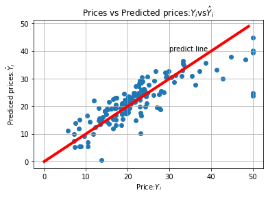
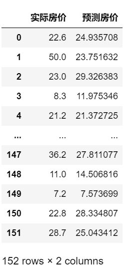
这是数据集的截图目录背景描述数据说明车型对照:燃料类型对照:老规矩,第一步先导入用到的库第二步,读入数据:第三步,数据预处理第四步:对数据的分析第五步:模型建立前的准备工作第六步:多元线性回归模型的建立第七步:随机森林模型的建立问题:背景描述本数据爬取自印度最大的二手车交易平台CARS24,包含8000+该平台上交易车辆的关键评估信息。CARS24成立于2015年,总部位于印度古尔冈,是一个在印度
- Java开发中,spring mvc 的线程怎么调用?
小麦麦子
springmvc
今天逛知乎,看到最近很多人都在问spring mvc 的线程http://www.maiziedu.com/course/java/ 的启动问题,觉得挺有意思的,那哥们儿问的也听仔细,下面的回答也很详尽,分享出来,希望遇对遇到类似问题的Java开发程序猿有所帮助。
问题:
在用spring mvc架构的网站上,设一线程在虚拟机启动时运行,线程里有一全局
- maven依赖范围
bitcarter
maven
1.test 测试的时候才会依赖,编译和打包不依赖,如junit不被打包
2.compile 只有编译和打包时才会依赖
3.provided 编译和测试的时候依赖,打包不依赖,如:tomcat的一些公用jar包
4.runtime 运行时依赖,编译不依赖
5.默认compile
依赖范围compile是支持传递的,test不支持传递
1.传递的意思是项目A,引用
- Jaxb org.xml.sax.saxparseexception : premature end of file
darrenzhu
xmlprematureJAXB
如果在使用JAXB把xml文件unmarshal成vo(XSD自动生成的vo)时碰到如下错误:
org.xml.sax.saxparseexception : premature end of file
很有可能时你直接读取文件为inputstream,然后将inputstream作为构建unmarshal需要的source参数。InputSource inputSource = new In
- CSS Specificity
周凡杨
html权重Specificitycss
有时候对于页面元素设置了样式,可为什么页面的显示没有匹配上呢? because specificity
CSS 的选择符是有权重的,当不同的选择符的样式设置有冲突时,浏览器会采用权重高的选择符设置的样式。
规则:
HTML标签的权重是1
Class 的权重是10
Id 的权重是100
- java与servlet
g21121
servlet
servlet 搞java web开发的人一定不会陌生,而且大家还会时常用到它。
下面是java官方网站上对servlet的介绍: java官网对于servlet的解释 写道
Java Servlet Technology Overview Servlets are the Java platform technology of choice for extending and enha
- eclipse中安装maven插件
510888780
eclipsemaven
1.首先去官网下载 Maven:
http://www.apache.org/dyn/closer.cgi/maven/binaries/apache-maven-3.2.3-bin.tar.gz
下载完成之后将其解压,
我将解压后的文件夹:apache-maven-3.2.3,
并将它放在 D:\tools目录下,
即 maven 最终的路径是:D:\tools\apache-mave
- jpa@OneToOne关联关系
布衣凌宇
jpa
Nruser里的pruserid关联到Pruser的主键id,实现对一个表的增删改,另一个表的数据随之增删改。
Nruser实体类
//*****************************************************************
@Entity
@Table(name="nruser")
@DynamicInsert @Dynam
- 我的spring学习笔记11-Spring中关于声明式事务的配置
aijuans
spring事务配置
这两天学到事务管理这一块,结合到之前的terasoluna框架,觉得书本上讲的还是简单阿。我就把我从书本上学到的再结合实际的项目以及网上看到的一些内容,对声明式事务管理做个整理吧。我看得Spring in Action第二版中只提到了用TransactionProxyFactoryBean和<tx:advice/>,定义注释驱动这三种,我承认后两种的内容很好,很强大。但是实际的项目当中
- java 动态代理简单实现
antlove
javahandlerproxydynamicservice
dynamicproxy.service.HelloService
package dynamicproxy.service;
public interface HelloService {
public void sayHello();
}
dynamicproxy.service.impl.HelloServiceImpl
package dynamicp
- JDBC连接数据库
百合不是茶
JDBC编程JAVA操作oracle数据库
如果我们要想连接oracle公司的数据库,就要首先下载oralce公司的驱动程序,将这个驱动程序的jar包导入到我们工程中;
JDBC链接数据库的代码和固定写法;
1,加载oracle数据库的驱动;
&nb
- 单例模式中的多线程分析
bijian1013
javathread多线程java多线程
谈到单例模式,我们立马会想到饿汉式和懒汉式加载,所谓饿汉式就是在创建类时就创建好了实例,懒汉式在获取实例时才去创建实例,即延迟加载。
饿汉式:
package com.bijian.study;
public class Singleton {
private Singleton() {
}
// 注意这是private 只供内部调用
private static
- javascript读取和修改原型特别需要注意原型的读写不具有对等性
bijian1013
JavaScriptprototype
对于从原型对象继承而来的成员,其读和写具有内在的不对等性。比如有一个对象A,假设它的原型对象是B,B的原型对象是null。如果我们需要读取A对象的name属性值,那么JS会优先在A中查找,如果找到了name属性那么就返回;如果A中没有name属性,那么就到原型B中查找name,如果找到了就返回;如果原型B中也没有
- 【持久化框架MyBatis3六】MyBatis3集成第三方DataSource
bit1129
dataSource
MyBatis内置了数据源的支持,如:
<environments default="development">
<environment id="development">
<transactionManager type="JDBC" />
<data
- 我程序中用到的urldecode和base64decode,MD5
bitcarter
cMD5base64decodeurldecode
这里是base64decode和urldecode,Md5在附件中。因为我是在后台所以需要解码:
string Base64Decode(const char* Data,int DataByte,int& OutByte)
{
//解码表
const char DecodeTable[] =
{
0, 0, 0, 0, 0, 0
- 腾讯资深运维专家周小军:QQ与微信架构的惊天秘密
ronin47
社交领域一直是互联网创业的大热门,从PC到移动端,从OICQ、MSN到QQ。到了移动互联网时代,社交领域应用开始彻底爆发,直奔黄金期。腾讯在过去几年里,社交平台更是火到爆,QQ和微信坐拥几亿的粉丝,QQ空间和朋友圈各种刷屏,写心得,晒照片,秀视频,那么谁来为企鹅保驾护航呢?支撑QQ和微信海量数据背后的架构又有哪些惊天内幕呢?本期大讲堂的内容来自今年2月份ChinaUnix对腾讯社交网络运营服务中心
- java-69-旋转数组的最小元素。把一个数组最开始的若干个元素搬到数组的末尾,我们称之为数组的旋转。输入一个排好序的数组的一个旋转,输出旋转数组的最小元素
bylijinnan
java
public class MinOfShiftedArray {
/**
* Q69 旋转数组的最小元素
* 把一个数组最开始的若干个元素搬到数组的末尾,我们称之为数组的旋转。输入一个排好序的数组的一个旋转,输出旋转数组的最小元素。
* 例如数组{3, 4, 5, 1, 2}为{1, 2, 3, 4, 5}的一个旋转,该数组的最小值为1。
*/
publ
- 看博客,应该是有方向的
Cb123456
反省看博客
看博客,应该是有方向的:
我现在就复习以前的,在补补以前不会的,现在还不会的,同时完善完善项目,也看看别人的博客.
我刚突然想到的:
1.应该看计算机组成原理,数据结构,一些算法,还有关于android,java的。
2.对于我,也快大四了,看一些职业规划的,以及一些学习的经验,看看别人的工作总结的.
为什么要写
- [开源与商业]做开源项目的人生活上一定要朴素,尽量减少对官方和商业体系的依赖
comsci
开源项目
为什么这样说呢? 因为科学和技术的发展有时候需要一个平缓和长期的积累过程,但是行政和商业体系本身充满各种不稳定性和不确定性,如果你希望长期从事某个科研项目,但是却又必须依赖于某种行政和商业体系,那其中的过程必定充满各种风险。。。
所以,为避免这种不确定性风险,我
- 一个 sql优化 ([精华] 一个查询优化的分析调整全过程!很值得一看 )
cwqcwqmax9
sql
见 http://www.itpub.net/forum.php?mod=viewthread&tid=239011
Web翻页优化实例
提交时间: 2004-6-18 15:37:49 回复 发消息
环境:
Linux ve
- Hibernat and Ibatis
dashuaifu
Hibernateibatis
Hibernate VS iBATIS 简介 Hibernate 是当前最流行的O/R mapping框架,当前版本是3.05。它出身于sf.net,现在已经成为Jboss的一部分了 iBATIS 是另外一种优秀的O/R mapping框架,当前版本是2.0。目前属于apache的一个子项目了。 相对Hibernate“O/R”而言,iBATIS 是一种“Sql Mappi
- 备份MYSQL脚本
dcj3sjt126com
mysql
#!/bin/sh
# this shell to backup mysql
#
[email protected] (QQ:1413161683 DuChengJiu)
_dbDir=/var/lib/mysql/
_today=`date +%w`
_bakDir=/usr/backup/$_today
[ ! -d $_bakDir ] && mkdir -p
- iOS第三方开源库的吐槽和备忘
dcj3sjt126com
ios
转自
ibireme的博客 做iOS开发总会接触到一些第三方库,这里整理一下,做一些吐槽。 目前比较活跃的社区仍旧是Github,除此以外也有一些不错的库散落在Google Code、SourceForge等地方。由于Github社区太过主流,这里主要介绍一下Github里面流行的iOS库。 首先整理了一份
Github上排名靠
- html wlwmanifest.xml
eoems
htmlxml
所谓优化wp_head()就是把从wp_head中移除不需要元素,同时也可以加快速度。
步骤:
加入到function.php
remove_action('wp_head', 'wp_generator');
//wp-generator移除wordpress的版本号,本身blog的版本号没什么意义,但是如果让恶意玩家看到,可能会用官网公布的漏洞攻击blog
remov
- 浅谈Java定时器发展
hacksin
java并发timer定时器
java在jdk1.3中推出了定时器类Timer,而后在jdk1.5后由Dou Lea从新开发出了支持多线程的ScheduleThreadPoolExecutor,从后者的表现来看,可以考虑完全替代Timer了。
Timer与ScheduleThreadPoolExecutor对比:
1.
Timer始于jdk1.3,其原理是利用一个TimerTask数组当作队列
- 移动端页面侧边导航滑入效果
ini
jqueryWebhtml5cssjavascirpt
效果体验:http://hovertree.com/texiao/mobile/2.htm可以使用移动设备浏览器查看效果。效果使用到jquery-2.1.4.min.js,该版本的jQuery库是用于支持HTML5的浏览器上,不再兼容IE8以前的浏览器,现在移动端浏览器一般都支持HTML5,所以使用该jQuery没问题。HTML文件代码:
<!DOCTYPE html>
<h
- AspectJ+Javasist记录日志
kane_xie
aspectjjavasist
在项目中碰到这样一个需求,对一个服务类的每一个方法,在方法开始和结束的时候分别记录一条日志,内容包括方法名,参数名+参数值以及方法执行的时间。
@Override
public String get(String key) {
// long start = System.currentTimeMillis();
// System.out.println("Be
- redis学习笔记
MJC410621
redisNoSQL
1)nosql数据库主要由以下特点:非关系型的、分布式的、开源的、水平可扩展的。
1,处理超大量的数据
2,运行在便宜的PC服务器集群上,
3,击碎了性能瓶颈。
1)对数据高并发读写。
2)对海量数据的高效率存储和访问。
3)对数据的高扩展性和高可用性。
redis支持的类型:
Sring 类型
set name lijie
get name lijie
set na
- 使用redis实现分布式锁
qifeifei
在多节点的系统中,如何实现分布式锁机制,其中用redis来实现是很好的方法之一,我们先来看一下jedis包中,有个类名BinaryJedis,它有个方法如下:
public Long setnx(final byte[] key, final byte[] value) {
checkIsInMulti();
client.setnx(key, value);
ret
- BI并非万能,中层业务管理报表要另辟蹊径
张老师的菜
大数据BI商业智能信息化
BI是商业智能的缩写,是可以帮助企业做出明智的业务经营决策的工具,其数据来源于各个业务系统,如ERP、CRM、SCM、进销存、HER、OA等。
BI系统不同于传统的管理信息系统,他号称是一个整体应用的解决方案,是融入管理思想的强大系统:有着系统整体的设计思想,支持对所有
- 安装rvm后出现rvm not a function 或者ruby -v后提示没安装ruby的问题
wudixiaotie
function
1.在~/.bashrc最后加入
[[ -s "$HOME/.rvm/scripts/rvm" ]] && source "$HOME/.rvm/scripts/rvm"
2.重新启动terminal输入:
rvm use ruby-2.2.1 --default
把当前安装的ruby版本设为默