原文: https://medium.com/blockchannel/on-value-velocity-and-monetary-theory-a-new-approach-to-cryptoasset-valuations-32c9b22e3b6f
作者: Alex Evans
VOLT: A Two-Asset Model with Endogenous Velocity
VOLT: 内生流通速度的双资产模型
In this section, I present an alternative cryptoasset valuation methodology that attempts to remedy the key problems identified in the last section. I model a fictitious utility token, VOLT, which can be exchanged by households to buy electricity at below-retail rates. Please note that while there are numerous projects targeting related use cases, this model in no way references these (it’s an entirely made-up example intended for illustrative purposes).
在这一节中,我提出了一种替代的密码资产评估方法,试图解决上一节中所识别出的关键问题。我建立了一个虚拟的实用(utility)代币,VOLT,它可以由家庭以低于零售价格的价格购买电力。请注意,虽然有许多项目针对相关的用例,但是这一模型没有引用它们(这是一个完全虚构的示例,用于说明的目的)。
The token is embedded in an economy with one good (electricity) and two assets: VOLT and a store-of-value asset that has a given expected rate of annual return. This is a frictional economy wherein users start with a fixed dollar amount at the beginning of each year in the store-of-value asset and must transfer their deposits to VOLT in order to finance their consumption of electricity, incurring transaction costs with each transfer. Note: You can select the store-of-value asset to be your favorite SoV cryptoasset or fiat-denominated security. This choice is of little importance to the functioning of the model as presented, except to the extent that it impacts your forecasted transaction costs.
代币内嵌在一个拥有一种货物(电力)和两种资产的经济中: VOLT 和一种具有给定预期年回报率的价值存储资产。这是一个有摩擦性的经济,用户在每年开始时有固定美元金额的价值存储资产,并且必须将他们的存款转换到VOLT ,以便为他们的电力消费提供资金,并在每次转账时产生交易成本。注意:您可以选择存储价值资产是哪一种,是你喜欢的SoV(Stock of Value, 价值存储)加密资产,或是法币计价的证券。这一选择对所描述的模型的运作没有什么大影响,除非它影响到你对交易成本的预期。
I model VOLT ‘money demand’ using the Baumol-Tobin “cash inventories” approach. Given that this method is slightly more involved than the INET approach, I pause to explain the key intuitions and underlying formulas before moving on to the actual model.
我用Baumol-Tobin的 “货币存货” 的思路来对VOLT的“货币需求”进行建模。考虑到这种方法比INET方法稍微复杂一些,我先停下来解释关键的直观观念和基本的公式,然后再转向实际的模型。
Total spending, Y, is the amount (in USD) that users plan to spend on VOLT each year. This can be thought of as the total GDP of the VOLT economy. Users spend Y uniformly throughout the year. R is the expected return on the store of value asset. C is the transaction cost of moving balances from the SoV asset to VOLT. N is the number of transfers that users of VOLT complete each year to ensure smooth consumption of electricity.
总花费,Y,是用户计划每年在VOLT上花费的金额(用美元表示)。这可以被看作是VOLT 经济体的总GDP。用户整年总共花费了Y。R是价值存储资产的预期收益。C是从 SoV 资产换为VOLT的交易成本。N是每年为确保对电力的平稳消耗,VOLT的用户所完成的交易量。
Users thus pay CN in transaction fees each year. The average money balance held in VOLT each year is Y/2N. The return that VOLT users forgo each year is RY/2N. Therefore, users select N, subject to Y, R, and C, in order to minimize their total cost function: RY/2N + CN. Taking the derivative of the total cost function with respect to N, we have:
因此,用户每年支付CN的交易费用。VOLT 每年的平均余额为Y/2N。VOLT 用户每年放弃的回报是RY/2N。因此,用户选择N,限定Y、R和C,以使其总成本函数最小化: RY/2N + CN。求总成本函数对N的导数,我们得到:
etting this equal to zero and solving for N we obtain the cost-minimizing N value of:
将它的值设为0, 然后求解N的值,我们得到让成本最小化的N的值为:
Finally, to get our money demand curve in terms of Y, C, and R, we plug the cost-minimizing N value back into the average money balance formula (Y/2N). We can now formulate our money demand function as:
最后,为了获得货币需求曲线,用Y, C和R来表示,我们把使成本最小化的N值代回到平均货币资产的公式(Y/2N)。现在我们可以把货币需求的方程写成:
We can thus say that VOLT ‘money demanded’ is equal to the cost-minimizing VOLT balance that users hold each year, which is a function of the GDP that the VOLT economy facilitates, the expected rate of return on the store-of-value asset, and the cost per transaction.
因此我们可以说,VOLT的“货币需求”等于用户每年所持有的让成本最小化的VOLT余额,这是VOLT 经济所产生的GDP、价值存储资产的预期回报率以及每笔交易的成本的一个函数。
Incidentally, we now have the tools at our disposal to formulate a definition of velocity without direct reference to the other monetary term in the equation of exchange, M. Velocity here is equal to the annual GDP, Y, of the VOLT economy over the demand for VOLT balances (the cost-minimizing average balance), or, equivalently, two times the optimal number of transfers, 2N. In other words, if a user transfers one large balance at the start of the year, each VOLT token turns over twice: Once when the user trades her SoV balance for VOLT and again when she exchanges it for electricity. If she buys in two times for half of the amount each time, each VOLT turns over four times, and so forth. Equipped with this definition, we can abandon the fixed-velocity approach of INET and instead project velocity endogenously alongside money demand as a function of Y, R, and C. Note this is equivalent to saying that ‘money demanded’ is equal to GDP over velocity, implying that our final result should still conform to MV=PT.
另外, 我们现在有工具能够形成对流通速度的定义,而不直接引用货币交换方程式中的其它货币术语,M.。流通速度等于:Y -- VOLT经济的年度GDP除以对VOLT额度的需求(成本最小化的平均余额), 或者等价地,最优交易次数的两倍,2N。换句话说,如果用户在年初时进行了一次大额兑换,那么每一个VOLT代币都会翻转两遍: 一次,当用户用她的“SoV”的额度交换VOLT时,l以及当她把VOLT换成电的时候。如果她分了两次购买,每次买一半,那么每个VOLT代币都要流转四次,如此等等。有了这个定义, 我们可以放弃INET模型中的固定流通速度的思路, 而是内生地衡量流通速度,将货币需求作为Y, R和C的函数。注意,这相当于说“货币需求”等于国内生产总值除以流通速度, 这意味着我们的最终结果仍应符合MV = PQ(原作似乎有误,为MV=PT)。
The model I use in the next section can be found here: https://docs.google.com/spreadsheets/d/1a1SzF2H1Y3twTvqAlGAwm8Q2jG-CPnP1Q-7qopN-4LE/edit#gid=428912142
下一节我用到的模型在这里可以找到: https://docs.google.com/spreadsheets/d/1a1SzF2H1Y3twTvqAlGAwm8Q2jG-CPnP1Q-7qopN-4LE/edit#gid=428912142
I would appreciate reporting of any issues you find with the model (especially mechanical problems/bugs), so I can update the sheet to work for everyone else.
如果你发现模型有任何问题(尤其是原理问题/bug),欢迎告诉我,这样我就可以更新这张表,让它对其他人也有用。
Step 1: VOLT Supply Schedule
步骤1: VOLT 供应安排
Despite the departure on other points, we still need to project both supply for VOLT tokens and residential electricity facilitated by the VOLT economy. Thankfully, Chris’ shoulders are there for us to stand on and I follow a virtually identical approach. With respect to money supply, the only theoretical difference is that I explicitly assume VOLT will have no HODLers as they will instead opt to hold the store-of-value asset (i.e. VOLT users are risk-averse). What is interesting about this point is that, in the model, each of the three functions of money is performed by a different asset: We have a separate Store-of-Value asset, while VOLT is the medium of exchange and USD is the internal unit of account. Reality will, of course, be more complicated.
尽管在其他方面有所不同,但我们仍然需要规划提供VOLT 代币供应和为VOLT经济体用到的电力供应。幸好我们可以站在Chris的肩膀上,我也遵循了一种几乎相同的思路。关于货币供应,唯一的理论区别是,我明确地假设了 VOLT没有坚定持有者(HODlers),因为他们将会选择持有价值储存的资产(即,VOLT用户是风险规避型的)。有趣的是,在模型中,货币的三个功能都是由不同的资产来执行的:我们有一个单独的价值存储资产,而 VOLT 是交换媒介,而美元是内部的记账单位。当然,现实会更复杂。
I model a supply of 100K VOLT, 10% of which is issued to founders, vesting at 25% annually starting after a one-year cliff. Another 10% is issued to the foundation, of which 20% is spent annually and returned to circulation. Unlike INET, I model VOLT supply as inflationary, growing at a 3% annual rate. This is arbitrary and included mainly for variety’s sake.
我的建模中,有100K VOLT 的供应量,其中10%是发给创始人的,在一年的锁定期之后,每年以25%的比例出售。另外10%的资金被发放给基金会,其中每年花费20%的资金用于花费,重新进入市场流通。与INET不同的是,我定义 VOLT 的供应方式是通货膨胀型的,以每年3%的速度增长。这是任意的,主要是为了多样化的缘故而设定。
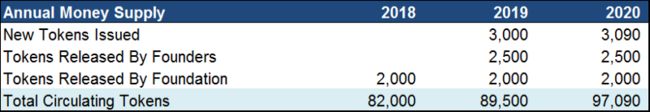
Total VOLT tokens in circulation are determined by the tokens already circulating, plus any tokens released by the founders or the VOLT foundation, plus new tokens created by the inflation mechanism each year.
已经流通的代币,加上创始人或VOLT 基金会释放的代币,再加上每年由通货膨胀机制创造的新的代币,决定了市场流通中VOLT代币的总数量。
Step 2: The VOLT Electricity Demand
步骤2: VOLT 电力需求
Note: For the electricity market, please open the notes in the assumption cells (highlighted on the top right of each cell) to see citations and additional notes. My aim here is to arrive at a value for GDP for the rest of the model to work, not to make any sort of claim about electricity markets. There are undoubtedly significant errors and oversimplifications in the assumptions.
注意:对于电力市场,请在假设的单元格(每个单元的右上方高亮显示)中打开注释,以查看引用和附加的说明。我在这里的目标,是得到一个GDP的值,能够让模型的其余部分可以生效,而不是要对电力市场提出任何批评。毫无疑问,在假设中会存在明显的错误和过度简化之处。
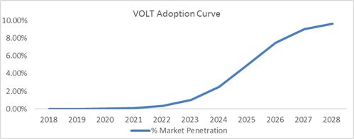
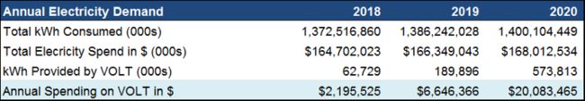
First, I assume a retail electricity price of $0.12 per kWh. I project this to stay flat as retail electricity prices have been relatively stable in recent years. I assume VOLT users can purchase electricity at $0.035 per kWh, an average price across U.S. wholesale markets. Again, I forecast no growth or decline in this price through 2028. Average kWh consumption per U.S. household was 10,766 kWh per year in 2017. Again, I project no change in this going forward. There were approximately 126 million U.S. households in 2017, which I assume will grow at 1% annually through 2028. To simplify things, VOLT is assumed to only be available in the U.S and to be capable of addressing 10% of the U.S. residential electricity market at peak penetration. To avoid overestimating market penetration in earlier years (and underestimating in later years), I follow Chris in projecting an S-curve for adoption. This curve has VOLT entering ‘hypergrowth’ starting in 2023, with a deceleration in the rate of growth as VOLT approaches market saturation and maturity over time.
首先,我假设零售价为每千瓦时(kWh)0.12美元。由于近年来零售电价相对稳定,所以我计划保持不变。我假设VOLT用户可以以每千瓦时0.035美元的价格购买电力,这是美国批发市场的平均价格。同样,我预计这个价格不会在2028年之前增长或下降。2017年,美国家庭平均每年的电力消费为10, 766千瓦时。同样,我在这方面没有改变。2017年,美国大约有1.26亿户家庭,我估计,到2028年,美国家庭的年增长率将达到1%。为了简化,我们认为VOLT代币只在美国可用, 在峰值时,会在美国住宅电力市场中,占到10%。为了避免在早期高估市场的渗透率(以及在以后的几年里低估了),我跟随Chris的思路设计了一条S曲线,以供采用。这条曲线从2023年开始进入“超级增长”,随着VOLT接近市场饱和和成熟,它的增长速度将会减慢。
Using the adoption curve, I estimate VOLT to capture a given percentage of kWh consumed by households in the US each year. This kWh share is multiplied by the wholesale electricity price to derive a value for annual spending on VOLT (i.e. VOLT’s ‘GDP’).
利用这条曲线,我估计VOLT可以占据美国家庭每年消费的kWh的一定百分比。这一千瓦时的份额乘以批发电价,得到每年花费在VOLT的价值 (即VOLT 的“GDP”)。
Again, the numbers are exclusively illustrative. If we needed to be more precise, for example, we might project adoption on a state-by-state or county-by-county basis (real-world electricity markets are highly localized) and specify a separate S-curve for each market.
再说一遍,这些数字只是用于说明的作用。如果我们需要更精确的话,比如,我们可以在州或县的基础上进行估计(现实世界的电力市场是高度本地化的),并为每个市场指定一条单独的S曲线。
Step 3: Money Demand for VOLT Tokens
步骤3: VOLT 代币的货币需求
To create the VOLT demand curve, I assume an expected rate of return on the store-of-value asset, a given initial transaction cost, and a transaction cost decline schedule.
为了创建VOLT需求曲线,我假定了价值存储资产的预期回报率,给定的初始交易成本,以及交易成本下降的时间表。
I assume a store-of-value asset with an expected return of 5% per year. Given that this essentially functions as a risk-free rate of return in our model, I would consider it quite an aggressive assumption (this just captures what I see as optimistic cryptoasset return expectations). You are obviously welcome (if not advised) to bring this value closer to a 3-month Treasury Bill (1.41% at the time of writing) or some other proxy of the risk-free rate (but remember to think about possible impacts on corresponding transaction cost assumptions). It may also be helpful to model some change in this value over time. However, ‘expectations’ are hard to project, so I just straight-line the value through 2028. I would love to see some debate on how to best handle this set of assumptions.
我假设是一种价值存储资产的预期年回报率为5%。考虑到这本质上是我们模型中的无风险回报率,我认为这是一个相当激进的假设(这恰好正是我所认为对加密资产回报预期的乐观估计)。也当然欢迎(如果不是建议的话)你把这个值设为接近3个月国债(在撰写本文时1.41%)或其他代理的无风险利率(但是记住考虑可能影响相应的交易成本的假设)。随着时间的推移,对这个值进行建模也会有所帮助。然而,“期望”是很难推断的,所以我只是把它的价值用到了2028年。我很乐意看到一些关于如何最好地处理这一系列假设的辩论。
Transaction costs in the initial year are assumed to be $20 per transfer, which is arguably an underestimation. Remember that this number is a fully-loaded representation of friction in the VOLT economy. These costs could include (but are not limited to): network transaction fees (for example, average BTC transaction fees were at $30 and Ethereum’s average gas cost at $1.1 at the time of writing), exchange fees and spreads (e.g. Bittrex charges 0.25% commission on trades), other costs resulting from illiquidity, any instability (real or anticipated) motivating the holding of precautionary VOLT balances to safeguard smooth consumption, the extent to which any given transaction constitutes a taxable event in the jurisdiction in question, time waiting for confirmations, implicit costs relating to asset custody and counterparty risk, inconvenience and cognitive load. I expect the ‘mental’ friction component to be the most significant for an average user. The better we can estimate and forecast the transaction cost parameter, the more accurate our model will be, so I would appreciate suggestions and debate on this point as well.
最初一年的交易成本假定为每次货币转换为20美元,这可以说是低估了。请记住,这个数字是VOLT 经济中一个完全负载的摩擦表示。这些成本可能包括(但不限于):网络交易费用(例如,平均BTC交易费用在30美元, Ethereum平均gas成本在撰写本文时1.1美元), 交易所费用和传播(如Bittrex收取0.25%的交易佣金),其它由于流动性不足产生的费用,任何不稳定(实际或预期的)会促使人们出于防御在账户中持有一定的VOLT,用于维护电力的顺利消费, 任何特定的交易在管辖范围内的应税事件的程度, 等待确认, 与资产托管和交易对手风险相关的隐性风险, 不便和认知负荷。我认为“心理”摩擦部分,对一般用户来说是最重要的。我们对交易成本参数的估计和预测越好,我们的模型就越准确,因此我也会对这一点提出建议和讨论。
As far as projecting how transaction costs will behave in the future, my main interest here is to numerically test the velocity thesis that states that utility token values will collapse alongside transaction costs in a frictionless future. To that aim, I find it most conceptually correct to model transaction cost declines in a similar manner to token adoption, using the familiar S-Curve. Here, friction could be said to decline for technological reasons (e.g. second-layer scaling solutions and cross-chain atomic swaps) as well as behavioral reasons (users become more comfortable with using cryptoassets in their daily lives). As such, transaction costs decline very slowly in initial years, but begin declining aggressively in 2023, the same year that VOLT enters hypergrowth (i.e. when mainstream users, not just early adopters, begin using the network as per the traditional S-curve “diffusion of innovation” theory). Ultimately, I assume a miniscule transaction cost in the final year, equal to $0.36 (essentially zero relative to the projected size of the average VOLT transfer of $270K in 2028).
在预测交易成本在未来会表现如何时,我的主要兴趣是通过对流通速度的论点进行数值测试,即在无摩擦的未来中,实用代币的价值将与交易成本一起崩溃。为了这个目的,我发现使用类似的S-Curve,采用与构建代币使用模型类似的方式对交易成本的下降进行建模,在概念上是正确的。在这里,可以说由于技术原因(例如第二层的伸缩解决方案和跨链的原子交换)以及行为原因(用户在日常生活中使用加密资产变得更加舒适),可能会导致摩擦的减少。因此,在最初几年,交易成本的下降非常缓慢,但在2023年,即VOLT进入高速增长时(根据传统的S曲线“创新扩散”理论,主流用户,而不仅仅是早期的使用者开始使用这一网络),交易成本开始大幅下降。最终,我假设在最后一年的交易成本很小,等于0.36美元(相对于2028年VOLT达到的平均交易额为$270K的规模来说,可以视作为零)。
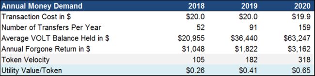
Based on the formulas previously laid out, I calculate the optimal number of transfers per year as a function of VOLT GDP, the expected rate of return on the SoV asset, and the transaction cost. The amount transferred each time is the total spending in VOLT (VOLT GDP) over the number of transfers for that year. Similarly, the average VOLT held (VOLT demand function) is VOLT GDP over two times the number of transfers. This number times the expected rate of return on the SoV asset is the amount of return VOLT users forgo each year.
根据之前列出的公式,我计算出每年 作为VOLT GDP(VOLT)的函数的每年最优交易量,SoV资产的期望收益率,以及交易成本。每一次交易转账的金额,是用当年 VOLT 的消费总额(VOLT GDP),除以当年的交易转账数量。同样的,VOLT的平均持有量(VOLT需求函数)是VOLT的GDP除以交易数量的两倍。这个数字乘以SoV资产的预期回报率,是用户每年放弃的回报率。
We calculate velocity directly as VOLT GDP over the annual VOLT money demand (average VOLT balance held). Remember that this can also be calculated as two times the number of transfers. Finally, utility value is calculated as Money Demanded/Money Supplied, or average VOLT balance held over the number of circulating VOLT tokens (MV=PQ solution). As such, we can restate the solution as VOLT GDP over the product of VOLT tokens in the float and velocity for that year.
我们计算的流通速度,是直接用VOLT GDP除以年度的VOLT 货币需求(VOLT的账户平均持有量)。记住,这也可以计算为转账数量的两倍。最后,效用价值被计算为货币需求/货币供应,或者说VOLT账户的平均值除以VOLT代币的流动次数(MV=PQ解决方案)。因此,我们可以将答案重新表述为VOLT的GDP除以VOLT代币在那一年的流动数量和流通速度的乘积之后,得到的结果。
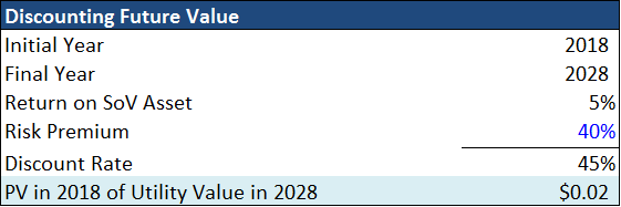
Finally, we discount the future utility value in 2028 back to 2018. The discount rate here differs slightly from INET, as we need to incorporate the risk-free rate (very high at 5%). Note that the resulting present value of $0.0244 in 2018 is more than ten times lower than per-token utility value for VOLT in that year. In other words, VOLT would have to be trading at an over a 90% discount to utility value in 2018 to yield a positive expected return for an investor intending to hold through 2028.
最后,我们将2028年的效用价值折算到2018年。这里的贴现率与INET略有不同,因为我们需要合并无风险利率(非常高的5%)。值得注意的是,到2018年,所产生的现值为0.0244美元,比当年VOLT的每代币的效用价值低10倍以上。换句话说,在2018年,VOLT的交易价格将比效用价值低90%以上,从而为有意持有到2028年的投资者带来积极的预期回报。
Step 4: Revisiting the Velocity Thesis
步骤4: 回顾货币流通速度的论点
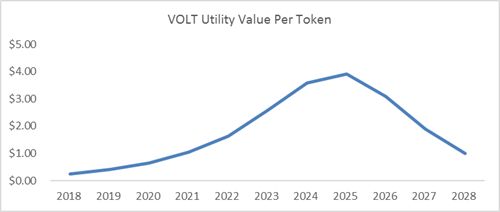
Plotting VOLT’s utility value over time, we see the velocity thesis’ core prediction in action as utility value peaks in 2025 and declines through 2028. Viewed through the prism of the INET model, this would appear strange as between 2025 and 2028 VOLT GDP grows nearly 100%, yet utility value per token declines.
将VOLT的效用价值随着时间的推移的变化画出来,我们看到货币流动性论点的核心预测是生效的,即2025年效用值达到峰值,并在2028年下降。从INET模型的角度来看,2025年至2028年VOLT的GDP增长接近100%,但单个代币的效用价值却下降,这看起来很奇怪。
This decline would not register in the INET approach, as demand for the token and demand for the resource are treated as one and the same. To explain what is happening under the hood, we return to the core prediction of the velocity thesis: As friction in the cryptoeconomy declines, demand for utility tokens falls as velocity growth overtakes PQ growth.
这种下降不会在INET的思路中出现,因为对资源的需求和对代币的需求被视为相同的一个东西。为了揭示到底发生了什么,我们回到了流通速度论点的核心预测: 随着在加密经济中的摩擦减少,对效用代币的需求下降,因为流通速度的增长超过了PQ的增长。
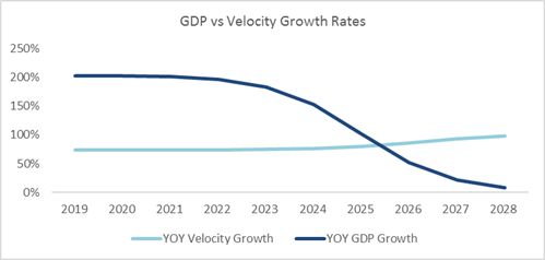
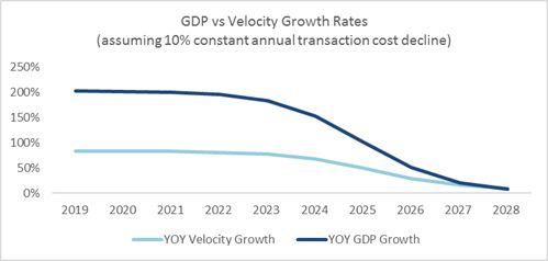
As we can see, despite the fact that during 2026–2028 GDP still grows at a rapid (albeit decelerating) pace, velocity grows even faster, putting downward pressure on price. Conceptually, even though users buy nearly double the amount of electricity using VOLT in 2028 than they do in 2025, they are able to satisfy this higher demand while still holding nearly two-thirds less in VOLT balances on average. In other words, collapsing transaction costs allow them to hold more of their wealth in the store-of-value asset, making many smaller transfers of VOLT as opposed to few larger ones to avoid forgoing return, leading to higher velocity/lower money demand. While velocity is a function of GDP, it is also a function of transaction costs, which begin to register dramatic declines after 2025. If, for example, we had projected transaction costs to decline at a steady rate, say 10%, the price decline would be delayed to 2028 as both velocity and GDP would fall together in the interim.
正如我们所看到的,尽管2026-2028年GDP仍在快速增长(尽管增速放缓),但流通速度的增长甚至更快,这给价格带来了下行压力。从概念上讲,即使用户在2028年购买的电量几乎是2025年的两倍,但他们在VOLT上的余额减少近三分之二的情况下,仍然能够满足这一更高的需求。换句话说,交易成本的大幅下滑使他们能够持有更多的价值存储代币,进行多次更小额度的VOLT交易转换而不是进行较少次数但额度更大的转换,以避免收益的损失,这导致了更高的货币流通速度,和更低的货币需求量。虽然流通速度是GDP的函数,但它也是交易成本的函数,交易成本在2025年之后开始急剧下降。例如,如果我们预测交易成本以稳定的速度下降,比如10%,价格下降将推迟到2028年,因为速度和GDP都将在这段时间内下降。
While we can deduce the strong correlation between velocity, VOLT GDP, and transaction costs just by looking at the formulas, the relation between GDP and utility value is what truly matters to our conclusion as per the velocity thesis.
虽然我们可以通过计算公式推导出流通速度、VOLT GDP和交易成本之间的强相关性,但根据流通速度的论点,对我们的结论而言GDP与效用值之间的关系才是真正重要的。
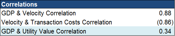
Here we see the how endogenous velocity allows us to decouple utility value from GDP growth. In the INET model, the correlation between GDP growth and INET value is a perfect 1:1 and the correlation between velocity and GDP growth is zero (velocity is fixed). In our model, the correlation between GDP growth and utility value is 0.34. This is what is driving the result.
在这里,我们可以看到内生的流通速度是如何让我们将效用值与GDP增长脱钩的。在INET模型中,GDP增长与INET的价值之间的相关性是一个完美的1:1,流通速度与GDP增长率之间的相关性为零(速度是固定的)。在我们的模型中,GDP增长与效用值的相关性为0.34。这就是导致结果的原因。
The final point to note about our results is that the utility value of VOLT largely depends on factors outside of VOLT’s ecosystem. Namely, expected returns and transaction costs.
最后要注意的是,VOLT 的效用值很大程度上取决于VOLT 的生态系统之外的因素。即预期收益和交易成本。
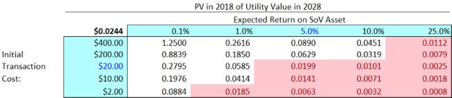
In the sensitivity analysis, we see that VOLT’s discounted future utility value varies significantly based on different inputs for C and R (values below our current discounted utility value projection are highlighted in red). This is where I would like to spend more time developing better estimates.
在敏感性分析(sensitivity analysis)中,我们看到 VOLT 的贴现未来效用值因C和R的不同输入而有很大的变动(低于我们预估贴现效用值的现值,用红色高亮显示)。我想在这上面花更多时间来优化,以便得到更好的估量。
Parting Thoughts 结语
Our valuation techniques are ultimately only as good as our accounting standards, measurement tools, and theoretical understanding of value. To that aim, I hope this piece has clarified some of the theoretical valuation debates unfolding in the investment community and has offered some helpful tools for modeling the value of cryptoassets. There are undoubtedly countless mistakes and simplifications in this approach that I hope subsequent discussion will illuminate. I look forward to these debates.
我们的评估技术的好坏,最终只会和我们的会计标准、测量工具和对价值的理论理解一样的水平。为了达到这个目的,我希望这篇文章对现在投资社区中的估值的理论争辩做了部分澄清,并提供了一些有用的工具用于加密资产的价值建模。毫无疑问,在这种方法中有无数的错误和简化,我希望后续的讨论中能够加以阐明。我期待着这些辩论。
Many thanks to Steven Mckie for helping me think through this piece, Oliver Beige for kindly sanity checking the economic logic, as well as everyone cited above for their thought-provoking work on cryptoasset valuations and beyond.
非常感谢Steven Mckie 在我思考这篇文章时的帮助, 感谢 Oliver Beige 帮助进行了经济学逻辑上的审查, 感谢上面所提到的所有的人,感谢他们在加密资产估值及其它事情上所做出的发人深省的研究。