一、图像分类2

二、GAN

三、DCGAN

一、图像分类2

Kaggle上的狗品种识别（ImageNet Dogs）
在本节中，我们将解决Kaggle竞赛中的犬种识别挑战，比赛的网址是https://www.kaggle.com/c/dog-breed-identification 在这项比赛中，我们尝试确定120种不同的狗。该比赛中使用的数据集实际上是著名的ImageNet数据集的子集。

# 在本节notebook中，使用后续设置的参数在完整训练集上训练模型，大致需要40-50分钟
# 请大家合理安排GPU时长，尽量只在训练时切换到GPU资源
# 也可以在Kaggle上访问本节notebook：
# https://www.kaggle.com/boyuai/boyu-d2l-dog-breed-identification-imagenet-dogs
import torch
import torch.nn as nn
import torch.optim as optim
import torchvision
import torchvision.transforms as transforms
import torchvision.models as models
import os
import shutil
import time
import pandas as pd
import random

# 设置随机数种子
random.seed(0)
torch.manual_seed(0)
torch.cuda.manual_seed(0)

1.1 整理数据集

我们可以从比赛网址上下载数据集，其目录结构为：

我们希望对数据进行整理，方便后续的读取，我们的主要目标是：

从训练集中划分出验证数据集，用于调整超参数。划分之后，数据集应该包含4个部分：划分后的训练集、划分后的验证集、完整训练集、完整测试集
对于4个部分，建立4个文件夹：train, valid, train_valid, test。在上述文件夹中，对每个类别都建立一个文件夹，在其中存放属于该类别的图像。前三个部分的标签已知，所以各有120个子文件夹，而测试集的标签未知，所以仅建立一个名为unknown的子文件夹，存放所有测试数据。
我们希望整理后的数据集目录结构为：

data_dir = '/home/kesci/input/Kaggle_Dog6357/dog-breed-identification'  # 数据集目录
label_file, train_dir, test_dir = 'labels.csv', 'train', 'test'  # data_dir中的文件夹、文件
new_data_dir = './train_valid_test'  # 整理之后的数据存放的目录
valid_ratio = 0.1  # 验证集所占比例

def mkdir_if_not_exist(path):
    # 若目录path不存在，则创建目录
    if not os.path.exists(os.path.join(*path)):
        os.makedirs(os.path.join(*path))
        
def reorg_dog_data(data_dir, label_file, train_dir, test_dir, new_data_dir, valid_ratio):
    # 读取训练数据标签
    labels = pd.read_csv(os.path.join(data_dir, label_file))
    id2label = {Id: label for Id, label in labels.values}  # (key: value): (id: label)

    # 随机打乱训练数据
    train_files = os.listdir(os.path.join(data_dir, train_dir))
    random.shuffle(train_files)    

    # 原训练集
    valid_ds_size = int(len(train_files) * valid_ratio)  # 验证集大小
    for i, file in enumerate(train_files):
        img_id = file.split('.')[0]  # file是形式为id.jpg的字符串
        img_label = id2label[img_id]
        if i < valid_ds_size:
            mkdir_if_not_exist([new_data_dir, 'valid', img_label])
            shutil.copy(os.path.join(data_dir, train_dir, file),
                        os.path.join(new_data_dir, 'valid', img_label))
        else:
            mkdir_if_not_exist([new_data_dir, 'train', img_label])
            shutil.copy(os.path.join(data_dir, train_dir, file),
                        os.path.join(new_data_dir, 'train', img_label))
        mkdir_if_not_exist([new_data_dir, 'train_valid', img_label])
        shutil.copy(os.path.join(data_dir, train_dir, file),
                    os.path.join(new_data_dir, 'train_valid', img_label))

    # 测试集
    mkdir_if_not_exist([new_data_dir, 'test', 'unknown'])
    for test_file in os.listdir(os.path.join(data_dir, test_dir)):
        shutil.copy(os.path.join(data_dir, test_dir, test_file),
                    os.path.join(new_data_dir, 'test', 'unknown'))

reorg_dog_data(data_dir, label_file, train_dir, test_dir, new_data_dir, valid_ratio)

1.2 图像增强

transform_train = transforms.Compose([
    # 随机对图像裁剪出面积为原图像面积0.08~1倍、且高和宽之比在3/4~4/3的图像，再放缩为高和宽均为224像素的新图像
    transforms.RandomResizedCrop(224, scale=(0.08, 1.0),  
                                 ratio=(3.0/4.0, 4.0/3.0)),
    # 以0.5的概率随机水平翻转
    transforms.RandomHorizontalFlip(),
    # 随机更改亮度、对比度和饱和度
    transforms.ColorJitter(brightness=0.4, contrast=0.4, saturation=0.4),
    transforms.ToTensor(),
    # 对各个通道做标准化，(0.485, 0.456, 0.406)和(0.229, 0.224, 0.225)是在ImageNet上计算得的各通道均值与方差
    transforms.Normalize([0.485, 0.456, 0.406], [0.229, 0.224, 0.225])  # ImageNet上的均值和方差
])

# 在测试集上的图像增强只做确定性的操作
transform_test = transforms.Compose([
    transforms.Resize(256),
    # 将图像中央的高和宽均为224的正方形区域裁剪出来
    transforms.CenterCrop(224),
    transforms.ToTensor(),
    transforms.Normalize([0.485, 0.456, 0.406], [0.229, 0.224, 0.225])
])

1.3 读取数据

# new_data_dir目录下有train, valid, train_valid, test四个目录
# 这四个目录中，每个子目录表示一种类别，目录中是属于该类别的所有图像
train_ds = torchvision.datasets.ImageFolder(root=os.path.join(new_data_dir, 'train'),
                                            transform=transform_train)
valid_ds = torchvision.datasets.ImageFolder(root=os.path.join(new_data_dir, 'valid'),
                                            transform=transform_test)
train_valid_ds = torchvision.datasets.ImageFolder(root=os.path.join(new_data_dir, 'train_valid'),
                                            transform=transform_train)
test_ds = torchvision.datasets.ImageFolder(root=os.path.join(new_data_dir, 'test'),
                                            transform=transform_test)

batch_size = 128
train_iter = torch.utils.data.DataLoader(train_ds, batch_size=batch_size, shuffle=True)
valid_iter = torch.utils.data.DataLoader(valid_ds, batch_size=batch_size, shuffle=True)
train_valid_iter = torch.utils.data.DataLoader(train_valid_ds, batch_size=batch_size, shuffle=True)
test_iter = torch.utils.data.DataLoader(test_ds, batch_size=batch_size, shuffle=False)  # shuffle=False

1.4 定义模型

这个比赛的数据属于ImageNet数据集的子集，我们使用微调的方法，选用在ImageNet完整数据集上预训练的模型来抽取图像特征，以作为自定义小规模输出网络的输入。

此处我们使用与训练的ResNet-34模型，直接复用预训练模型在输出层的输入，即抽取的特征，然后我们重新定义输出层，本次我们仅对重定义的输出层的参数进行训练，而对于用于抽取特征的部分，我们保留预训练模型的参数。

def get_net(device):
    finetune_net = models.resnet34(pretrained=False)  # 预训练的resnet34网络
    finetune_net.load_state_dict(torch.load('/home/kesci/input/resnet347742/resnet34-333f7ec4.pth'))
    for param in finetune_net.parameters():  # 冻结参数
        param.requires_grad = False
    # 原finetune_net.fc是一个输入单元数为512，输出单元数为1000的全连接层
    # 替换掉原finetune_net.fc，新finetuen_net.fc中的模型参数会记录梯度
    finetune_net.fc = nn.Sequential(
        nn.Linear(in_features=512, out_features=256),
        nn.ReLU(),
        nn.Linear(in_features=256, out_features=120)  # 120是输出类别数
    )
    return finetune_net

1.5 定义训练数据

def evaluate_loss_acc(data_iter, net, device):
    # 计算data_iter上的平均损失与准确率
    loss = nn.CrossEntropyLoss()
    is_training = net.training  # Bool net是否处于train模式
    net.eval()
    l_sum, acc_sum, n = 0, 0, 0
    with torch.no_grad():
        for X, y in data_iter:
            X, y = X.to(device), y.to(device)
            y_hat = net(X)
            l = loss(y_hat, y)
            l_sum += l.item() * y.shape[0]
            acc_sum += (y_hat.argmax(dim=1) == y).sum().item()
            n += y.shape[0]
    net.train(is_training)  # 恢复net的train/eval状态
    return l_sum / n, acc_sum / n
def train(net, train_iter, valid_iter, num_epochs, lr, wd, device, lr_period,
          lr_decay):
    loss = nn.CrossEntropyLoss()
    optimizer = optim.SGD(net.fc.parameters(), lr=lr, momentum=0.9, weight_decay=wd)
    net = net.to(device)
    for epoch in range(num_epochs):
        train_l_sum, n, start = 0.0, 0, time.time()
        if epoch > 0 and epoch % lr_period == 0:  # 每lr_period个epoch，学习率衰减一次
            lr = lr * lr_decay
            for param_group in optimizer.param_groups:
                param_group['lr'] = lr
        for X, y in train_iter:
            X, y = X.to(device), y.to(device)
            optimizer.zero_grad()
            y_hat = net(X)
            l = loss(y_hat, y)
            l.backward()
            optimizer.step()
            train_l_sum += l.item() * y.shape[0]
            n += y.shape[0]
        time_s = "time %.2f sec" % (time.time() - start)
        if valid_iter is not None:
            valid_loss, valid_acc = evaluate_loss_acc(valid_iter, net, device)
            epoch_s = ("epoch %d, train loss %f, valid loss %f, valid acc %f, "
                       % (epoch + 1, train_l_sum / n, valid_loss, valid_acc))
        else:
            epoch_s = ("epoch %d, train loss %f, "
                       % (epoch + 1, train_l_sum / n))
        print(epoch_s + time_s + ', lr ' + str(lr))

1.6 调参

num_epochs, lr_period, lr_decay = 20, 10, 0.1
lr, wd = 0.03, 1e-4
device = torch.device('cuda' if torch.cuda.is_available() else 'cpu')

net = get_net(device)
train(net, train_iter, valid_iter, num_epochs, lr, wd, device, lr_period, lr_decay)

1.7 在完整数据集上训练模型

# 使用上面的参数设置，在完整数据集上训练模型大致需要40-50分钟的时间
net = get_net(device)
train(net, train_valid_iter, None, num_epochs, lr, wd, device, lr_period, lr_decay)

1.8 对测试集分类并提交结果

用训练好的模型对测试数据进行预测。比赛要求对测试集中的每张图片，都要预测其属于各个类别的概率。

preds = []
for X, _ in test_iter:
    X = X.to(device)
    output = net(X)
    output = torch.softmax(output, dim=1)
    preds += output.tolist()
ids = sorted(os.listdir(os.path.join(new_data_dir, 'test/unknown')))
with open('submission.csv', 'w') as f:
    f.write('id,' + ','.join(train_valid_ds.classes) + '\n')
    for i, output in zip(ids, preds):
        f.write(i.split('.')[0] + ',' + ','.join(
            [str(num) for num in output]) + '\n')

二、GAN（Generative Adversarial Networks）

Throughout most of this book, we have talked about how to make predictions. In some form or another, we used deep neural networks learned mappings from data points to labels. This kind of learning is called discriminative learning, as in, we'd like to be able to discriminate between photos cats and photos of dogs. Classifiers and regressors are both examples of discriminative learning. And neural networks trained by backpropagation have upended everything we thought we knew about discriminative learning on large complicated datasets. Classification accuracies on high-res images has gone from useless to human-level (with some caveats) in just 5-6 years. We will spare you another spiel about all the other discriminative tasks where deep neural networks do astoundingly well.

But there is more to machine learning than just solving discriminative tasks. For example, given a large dataset, without any labels, we might want to learn a model that concisely captures the characteristics of this data. Given such a model, we could sample synthetic data points that resemble the distribution of the training data. For example, given a large corpus of photographs of faces, we might want to be able to generate a new photorealistic image that looks like it might plausibly have come from the same dataset. This kind of learning is called generative modeling.

Until recently, we had no method that could synthesize novel photorealistic images. But the success of deep neural networks for discriminative learning opened up new possibilities. One big trend over the last three years has been the application of discriminative deep nets to overcome challenges in problems that we do not generally think of as supervised learning problems. The recurrent neural network language models are one example of using a discriminative network (trained to predict the next character) that once trained can act as a generative model.

In 2014, a breakthrough paper introduced Generative adversarial networks (GANs) Goodfellow.Pouget-Abadie.Mirza.ea.2014, a clever new way to leverage the power of discriminative models to get good generative models. At their heart, GANs rely on the idea that a data generator is good if we cannot tell fake data apart from real data. In statistics, this is called a two-sample test - a test to answer the question whether datasets $X = {x_{1}, \dots, x_{n}}$ and $X^{'} = {x_{1}^{'}, \dots, x_{n}^{'}}$ were drawn from the same distribution. The main difference between most statistics papers and GANs is that the latter use this idea in a constructive way. In other words, rather than just training a model to say "hey, these two datasets do not look like they came from the same distribution", they use the two-sample test to provide training signals to a generative model. This allows us to improve the data generator until it generates something that resembles the real data. At the very least, it needs to fool the classifier. Even if our classifier is a state of the art deep neural network.

GAN

The GAN architecture is illustrated.As you can see, there are two pieces in GAN architecture - first off, we need a device (say, a deep network but it really could be anything, such as a game rendering engine) that might potentially be able to generate data that looks just like the real thing. If we are dealing with images, this needs to generate images. If we are dealing with speech, it needs to generate audio sequences, and so on. We call this the generator network. The second component is the discriminator network. It attempts to distinguish fake and real data from each other. Both networks are in competition with each other. The generator network attempts to fool the discriminator network. At that point, the discriminator network adapts to the new fake data. This information, in turn is used to improve the generator network, and so on.

The discriminator is a binary classifier to distinguish if the input x is real (from real data) or fake (from the generator). Typically, the discriminator outputs a scalar prediction o∈R for input x , such as using a dense layer with hidden size 1, and then applies sigmoid function to obtain the predicted probability D(x)=1/(1+e−o) . Assume the label y for the true data is 1 and 0 for the fake data. We train the discriminator to minimize the cross-entropy loss, i.e.,

minD{−ylogD(x)−(1−y)log(1−D(x))},

For the generator, it first draws some parameter z∈Rd from a source of randomness, e.g., a normal distribution z∼N(0,1) . We often call z as the latent variable. It then applies a function to generate x′=G(z) . The goal of the generator is to fool the discriminator to classify x′=G(z) as true data, i.e., we want D(G(z))≈1 . In other words, for a given discriminator D , we update the parameters of the generator G to maximize the cross-entropy loss when y=0 , i.e.,

maxG{−(1−y)log(1−D(G(z)))}=maxG{−log(1−D(G(z)))}.

If the discriminator does a perfect job, then D(x′)≈0 so the above loss near 0, which results the gradients are too small to make a good progress for the generator. So commonly we minimize the following loss:

minG{−ylog(D(G(z)))}=minG{−log(D(G(z)))},

which is just feed x′=G(z) into the discriminator but giving label y=1 .

To sum up, D and G are playing a "minimax" game with the comprehensive objective function:

minDmaxG{−Ex∼DatalogD(x)−Ez∼Noiselog(1−D(G(z)))}.

Many of the GANs applications are in the context of images. As a demonstration purpose, we are going to content ourselves with fitting a much simpler distribution first. We will illustrate what happens if we use GANs to build the world's most inefficient estimator of parameters for a Gaussian. Let's get started.

%matplotlib inline
import matplotlib.pyplot as plt
from torch.utils.data import DataLoader
from torch import nn
import numpy as np
from torch.autograd import Variable
import torch

1.1 Generate some 'real' data

Since this is going to be the world's lamest example, we simply generate data drawn from a Gaussian.

X=np.random.normal(size=(1000,2))
A=np.array([[1,2],[-0.1,0.5]])
b=np.array([1,2])
data=X.dot(A)+b

Let's see what we got. This should be a Gaussian shifted in some rather arbitrary way with mean b and covariance matrix ATA .

plt.figure(figsize=(3.5,2.5))
plt.scatter(X[:100,0],X[:100,1],color='red')
plt.show()
plt.figure(figsize=(3.5,2.5))
plt.scatter(data[:100,0],data[:100,1],color='blue')
plt.show()
print("The covariance matrix is\n%s" % np.dot(A.T, A))

生成型数据

batch_size=8
data_iter=DataLoader(data,batch_size=batch_size)

1.2 Generator

Our generator network will be the simplest network possible - a single layer linear model. This is since we will be driving that linear network with a Gaussian data generator. Hence, it literally only needs to learn the parameters to fake things perfectly.

class net_G(nn.Module):
    def __init__(self):
        super(net_G,self).__init__()
        self.model=nn.Sequential(
            nn.Linear(2,2),
        )
        self._initialize_weights()
    def forward(self,x):
        x=self.model(x)
        return x
    def _initialize_weights(self):
        for m in self.modules():
            if isinstance(m,nn.Linear):
                m.weight.data.normal_(0,0.02)
                m.bias.data.zero_()

1.3 Discriminator

For the discriminator we will be a bit more discriminating: we will use an MLP with 3 layers to make things a bit more interesting.

class net_D(nn.Module):
    def __init__(self):
        super(net_D,self).__init__()
        self.model=nn.Sequential(
            nn.Linear(2,5),
            nn.Tanh(),
            nn.Linear(5,3),
            nn.Tanh(),
            nn.Linear(3,1),
            nn.Sigmoid()
        )
        self._initialize_weights()
    def forward(self,x):
        x=self.model(x)
        return x
    def _initialize_weights(self):
        for m in self.modules():
            if isinstance(m,nn.Linear):
                m.weight.data.normal_(0,0.02)
                m.bias.data.zero_()

1.4 Training

First we define a function to update the discriminator.

# Saved in the d2l package for later use
def update_D(X,Z,net_D,net_G,loss,trainer_D):
    batch_size=X.shape[0]
    Tensor=torch.FloatTensor
    ones=Variable(Tensor(np.ones(batch_size))).view(batch_size,1)
    zeros = Variable(Tensor(np.zeros(batch_size))).view(batch_size,1)
    real_Y=net_D(X.float())
    fake_X=net_G(Z)
    fake_Y=net_D(fake_X)
    loss_D=(loss(real_Y,ones)+loss(fake_Y,zeros))/2
    loss_D.backward()
    trainer_D.step()
    return float(loss_D.sum())

The generator is updated similarly. Here we reuse the cross-entropy loss but change the label of the fake data from 0 to 1 .

# Saved in the d2l package for later use
def update_G(Z,net_D,net_G,loss,trainer_G):
    batch_size=Z.shape[0]
    Tensor=torch.FloatTensor
    ones=Variable(Tensor(np.ones((batch_size,)))).view(batch_size,1)
    fake_X=net_G(Z)
    fake_Y=net_D(fake_X)
    loss_G=loss(fake_Y,ones)
    loss_G.backward()
    trainer_G.step()
    return float(loss_G.sum())

Both the discriminator and the generator performs a binary logistic regression with the cross-entropy loss. We use Adam to smooth the training process. In each iteration, we first update the discriminator and then the generator. We visualize both losses and generated examples.

def train(net_D,net_G,data_iter,num_epochs,lr_D,lr_G,latent_dim,data):
    loss=nn.BCELoss()
    Tensor=torch.FloatTensor
    trainer_D=torch.optim.Adam(net_D.parameters(),lr=lr_D)
    trainer_G=torch.optim.Adam(net_G.parameters(),lr=lr_G)
    plt.figure(figsize=(7,4))
    d_loss_point=[]
    g_loss_point=[]
    d_loss=0
    g_loss=0
    for epoch in range(1,num_epochs+1):
        d_loss_sum=0
        g_loss_sum=0
        batch=0
        for X in data_iter:
            batch+=1
            X=Variable(X)
            batch_size=X.shape[0]
            Z=Variable(Tensor(np.random.normal(0,1,(batch_size,latent_dim))))
            trainer_D.zero_grad()
            d_loss = update_D(X, Z, net_D, net_G, loss, trainer_D)
            d_loss_sum+=d_loss
            trainer_G.zero_grad()
            g_loss = update_G(Z, net_D, net_G, loss, trainer_G)
            g_loss_sum+=g_loss
        d_loss_point.append(d_loss_sum/batch)
        g_loss_point.append(g_loss_sum/batch)
    plt.ylabel('Loss', fontdict={'size': 14})
    plt.xlabel('epoch', fontdict={'size': 14})
    plt.xticks(range(0,num_epochs+1,3))
    plt.plot(range(1,num_epochs+1),d_loss_point,color='orange',label='discriminator')
    plt.plot(range(1,num_epochs+1),g_loss_point,color='blue',label='generator')
    plt.legend()
    plt.show()
    print(d_loss,g_loss)
    
    Z =Variable(Tensor( np.random.normal(0, 1, size=(100, latent_dim))))
    fake_X=net_G(Z).detach().numpy()
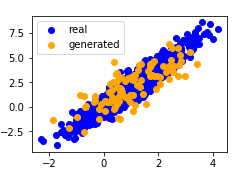
    plt.figure(figsize=(3.5,2.5))
    plt.scatter(data[:,0],data[:,1],color='blue',label='real')
    plt.scatter(fake_X[:,0],fake_X[:,1],color='orange',label='generated')
    plt.legend()
    plt.show()

Now we specify the hyper-parameters to fit the Gaussian distribution.

if __name__ == '__main__':
    lr_D,lr_G,latent_dim,num_epochs=0.05,0.005,2,20
    generator=net_G()
    discriminator=net_D()
    train(discriminator,generator,data_iter,num_epochs,lr_D,lr_G,latent_dim,data)

discriminator & generator

real & generated

1.5 Summary

-Generative adversarial networks (GANs) composes of two deep networks, the generator and the discriminator.
-The generator generates the image as much closer to the true image as possible to fool the discriminator, via maximizing the cross-entropy loss, i.e., maxlog(D(x′)) .
-The discriminator tries to distinguish the generated images from the true images, via minimizing the cross-entropy loss, i.e., min−ylogD(x)−(1−y)log(1−D(x)) .

三、DCGAN（Deep Convolutional Generative Adversarial Networks）

we introduced the basic ideas behind how GANs work. We showed that they can draw samples from some simple, easy-to-sample distribution, like a uniform or normal distribution, and transform them into samples that appear to match the distribution of some dataset. And while our example of matching a 2D Gaussian distribution got the point across, it is not especially exciting.

In this section, we will demonstrate how you can use GANs to generate photorealistic images. We will be basing our models on the deep convolutional GANs (DCGAN) introduced in :cite:Radford.Metz.Chintala.2015. We will borrow the convolutional architecture that have proven so successful for discriminative computer vision problems and show how via GANs, they can be leveraged to generate photorealistic images.

import matplotlib.pyplot as plt
from torch.utils.data import DataLoader
from torch import nn
import numpy as np
from torch.autograd import Variable
import torch
from torchvision.datasets import ImageFolder
from torchvision.transforms import transforms
import zipfile
cuda = True if torch.cuda.is_available() else False
print(cuda)

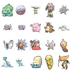
1.1 The Pokemon Dataset

The dataset we will use is a collection of Pokemon sprites obtained from pokemondb. First download, extract and load this dataset.

We resize each image into $64 \times 64$ . The ToTensor transformation will project the pixel value into $[0, 1]$ , while our generator will use the tanh function to obtain outputs in $[- 1, 1]$ . Therefore we normalize the data with $0.5$ mean and $0.5$ standard deviation to match the value range.

data_dir='/home/kesci/input/pokemon8600/'
batch_size=256
transform=transforms.Compose([
    transforms.Resize((64,64)),
    transforms.ToTensor(),
    transforms.Normalize((0.5,0.5,0.5),(0.5,0.5,0.5))
])
pokemon=ImageFolder(data_dir+'pokemon',transform)
data_iter=DataLoader(pokemon,batch_size=batch_size,shuffle=True)

Let's visualize the first 20 images.

fig=plt.figure(figsize=(4,4))
imgs=data_iter.dataset.imgs
for i in range(20):
    img = plt.imread(imgs[i*150][0])
    plt.subplot(4,5,i+1)
    plt.imshow(img)
    plt.axis('off')
plt.show()

pokemon

1.2 The Generator

The generator needs to map the noise variable z∈Rd , a length- d vector, to a RGB image with width and height to be 64×64 . In :numref:sec_fcn we introduced the fully convolutional network that uses transposed convolution layer (refer to :numref:sec_transposed_conv) to enlarge input size. The basic block of the generator contains a transposed convolution layer followed by the batch normalization and ReLU activation.

class G_block(nn.Module):
    def __init__(self, in_channels, out_channels, kernel_size=4,strides=2, padding=1):
        super(G_block,self).__init__()
        self.conv2d_trans=nn.ConvTranspose2d(in_channels, out_channels, kernel_size=kernel_size,
                                             stride=strides, padding=padding, bias=False)
        self.batch_norm=nn.BatchNorm2d(out_channels,0.8)
        self.activation=nn.ReLU()
    def forward(self,x):
        return self.activation(self.batch_norm(self.conv2d_trans(x)))

In default, the transposed convolution layer uses a kh=kw=4 kernel, a sh=sw=2 strides, and a ph=pw=1 padding. With a input shape of n′h×n′w=16×16 , the generator block will double input's width and height.

n′h×n′w=[(nhkh−(nh−1)(kh−sh)−2ph]×[(nwkw−(nw−1)(kw−sw)−2pw]=[(kh+sh(nh−1)−2ph]×[(kw+sw(nw−1)−2pw]=[(4+2×(16−1)−2×1]×[(4+2×(16−1)−2×1]=32×32.

Tensor=torch.cuda.FloatTensor
x=Variable(Tensor(np.zeros((2,3,16,16))))
g_blk=G_block(3,20)
g_blk.cuda()
print(g_blk(x).shape)

If changing the transposed convolution layer to a 4×4 kernel, 1×1 strides and zero padding. With a input size of 1×1 , the output will have its width and height increased by 3 respectively.

x=Variable(Tensor(np.zeros((2,3,1,1))))
g_blk=G_block(3,20,strides=1,padding=0)
g_blk.cuda()
print(g_blk(x).shape)

The generator consists of four basic blocks that increase input's both width and height from 1 to 32. At the same time, it first projects the latent variable into 64×8 channels, and then halve the channels each time. At last, a transposed convolution layer is used to generate the output. It further doubles the width and height to match the desired 64×64 shape, and reduces the channel size to 3 . The tanh activation function is applied to project output values into the (−1,1) range.

class net_G(nn.Module):
    def __init__(self,in_channels):
        super(net_G,self).__init__()

        n_G=64
        self.model=nn.Sequential(
            G_block(in_channels,n_G*8,strides=1,padding=0),
            G_block(n_G*8,n_G*4),
            G_block(n_G*4,n_G*2),
            G_block(n_G*2,n_G),
            nn.ConvTranspose2d(
                n_G,3,kernel_size=4,stride=2,padding=1,bias=False
            ),
            nn.Tanh()
        )
    def forward(self,x):
        x=self.model(x)
        return x


def weights_init_normal(m):
    classname = m.__class__.__name__
    if classname.find("Conv") != -1:
        torch.nn.init.normal_(m.weight.data, mean=0, std=0.02)
    elif classname.find("BatchNorm2d") != -1:
        torch.nn.init.normal_(m.weight.data, mean=1.0, std=0.02)
        torch.nn.init.constant_(m.bias.data, 0.0)

Generate a 100 dimensional latent variable to verify the generator's output shape.

x=Variable(Tensor(np.zeros((1,100,1,1))))
generator=net_G(100)
generator.cuda()
generator.apply(weights_init_normal)
print(generator(x).shape)

1.4 Discriminator

The discriminator is a normal convolutional network network except that it uses a leaky ReLU as its activation function. Given α∈[0,1] , its definition is

leaky ReLU

As it can be seen, it is normal ReLU if α=0 , and an identity function if α=1 . For α∈(0,1) , leaky ReLU is a nonlinear function that give a non-zero output for a negative input. It aims to fix the "dying ReLU" problem that a neuron might always output a negative value and therefore cannot make any progress since the gradient of ReLU is 0.

alphas = [0, 0.2, 0.4, .6]
x = np.arange(-2, 1, 0.1)
Y = [nn.LeakyReLU(alpha)(Tensor(x)).cpu().numpy()for alpha in alphas]
plt.figure(figsize=(4,4))
for y in Y:
    plt.plot(x,y)
plt.show()

plot~

The basic block of the discriminator is a convolution layer followed by a batch normalization layer and a leaky ReLU activation. The hyper-parameters of the convolution layer are similar to the transpose convolution layer in the generator block.

class D_block(nn.Module):
    def __init__(self,in_channels,out_channels,kernel_size=4,strides=2,
                 padding=1,alpha=0.2):
        super(D_block,self).__init__()
        self.conv2d=nn.Conv2d(in_channels,out_channels,kernel_size,strides,padding,bias=False)
        self.batch_norm=nn.BatchNorm2d(out_channels,0.8)
        self.activation=nn.LeakyReLU(alpha)
    def forward(self,X):
        return self.activation(self.batch_norm(self.conv2d(X)))

A basic block with default settings will halve the width and height of the inputs, as we demonstrated in :numref:sec_padding. For example, given a input shape nh=nw=16 , with a kernel shape kh=kw=4 , a stride shape sh=sw=2 , and a padding shape ph=pw=1 , the output shape will be:

设置参数

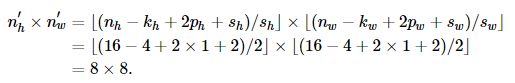
x = Variable(Tensor(np.zeros((2, 3, 16, 16))))
d_blk = D_block(3,20)
d_blk.cuda()
print(d_blk(x).shape)

The discriminator is a mirror of the generator.

class net_D(nn.Module):
    def __init__(self,in_channels):
        super(net_D,self).__init__()
        n_D=64
        self.model=nn.Sequential(
            D_block(in_channels,n_D),
            D_block(n_D,n_D*2),
            D_block(n_D*2,n_D*4),
            D_block(n_D*4,n_D*8)
        )
        self.conv=nn.Conv2d(n_D*8,1,kernel_size=4,bias=False)
        self.activation=nn.Sigmoid()
        # self._initialize_weights()
    def forward(self,x):
        x=self.model(x)
        x=self.conv(x)
        x=self.activation(x)
        return x

It uses a convolution layer with output channel 1 as the last layer to obtain a single prediction value.

x = Variable(Tensor(np.zeros((1, 3, 64, 64))))
discriminator=net_D(3)
discriminator.cuda()
discriminator.apply(weights_init_normal)
print(discriminator(x).shape)

1.5 Training

Compared to the basic GAN in :numref:sec_basic_gan, we use the same learning rate for both generator and discriminator since they are similar to each other. In addition, we change β1 in Adam (:numref:sec_adam) from 0.9 to 0.5 . It decreases the smoothness of the momentum, the exponentially weighted moving average of past gradients, to take care of the rapid changing gradients because the generator and the discriminator fight with each other. Besides, the random generated noise Z, is a 4-D tensor and we are using GPU to accelerate the computation.

def update_D(X,Z,net_D,net_G,loss,trainer_D):
    batch_size=X.shape[0]
    Tensor=torch.cuda.FloatTensor
    ones=Variable(Tensor(np.ones(batch_size,)),requires_grad=False).view(batch_size,1)
    zeros = Variable(Tensor(np.zeros(batch_size,)),requires_grad=False).view(batch_size,1)
    real_Y=net_D(X).view(batch_size,-1)
    fake_X=net_G(Z)
    fake_Y=net_D(fake_X).view(batch_size,-1)
    loss_D=(loss(real_Y,ones)+loss(fake_Y,zeros))/2
    loss_D.backward()
    trainer_D.step()
    return float(loss_D.sum())

def update_G(Z,net_D,net_G,loss,trainer_G):
    batch_size=Z.shape[0]
    Tensor=torch.cuda.FloatTensor
    ones=Variable(Tensor(np.ones((batch_size,))),requires_grad=False).view(batch_size,1)
    fake_X=net_G(Z)
    fake_Y=net_D(fake_X).view(batch_size,-1)
    loss_G=loss(fake_Y,ones)
    loss_G.backward()
    trainer_G.step()
    return float(loss_G.sum())


def train(net_D,net_G,data_iter,num_epochs,lr,latent_dim):
    loss=nn.BCELoss()
    Tensor=torch.cuda.FloatTensor
    trainer_D=torch.optim.Adam(net_D.parameters(),lr=lr,betas=(0.5,0.999))
    trainer_G=torch.optim.Adam(net_G.parameters(),lr=lr,betas=(0.5,0.999))
    plt.figure(figsize=(7,4))
    d_loss_point=[]
    g_loss_point=[]
    d_loss=0
    g_loss=0
    for epoch in range(1,num_epochs+1):
        d_loss_sum=0
        g_loss_sum=0
        batch=0
        for X in data_iter:
            X=X[:][0]
            batch+=1
            X=Variable(X.type(Tensor))
            batch_size=X.shape[0]
            Z=Variable(Tensor(np.random.normal(0,1,(batch_size,latent_dim,1,1))))

            trainer_D.zero_grad()
            d_loss = update_D(X, Z, net_D, net_G, loss, trainer_D)
            d_loss_sum+=d_loss
            trainer_G.zero_grad()
            g_loss = update_G(Z, net_D, net_G, loss, trainer_G)
            g_loss_sum+=g_loss

        d_loss_point.append(d_loss_sum/batch)
        g_loss_point.append(g_loss_sum/batch)
        print(
            "[Epoch %d/%d]  [D loss: %f] [G loss: %f]"
            % (epoch, num_epochs,  d_loss_sum/batch_size,  g_loss_sum/batch_size)
        )


    plt.ylabel('Loss', fontdict={ 'size': 14})
    plt.xlabel('epoch', fontdict={ 'size': 14})
    plt.xticks(range(0,num_epochs+1,3))
    plt.plot(range(1,num_epochs+1),d_loss_point,color='orange',label='discriminator')
    plt.plot(range(1,num_epochs+1),g_loss_point,color='blue',label='generator')
    plt.legend()
    plt.show()
    print(d_loss,g_loss)

    Z = Variable(Tensor(np.random.normal(0, 1, size=(21, latent_dim, 1, 1))),requires_grad=False)
    fake_x = generator(Z)
    fake_x=fake_x.cpu().detach().numpy()
    plt.figure(figsize=(14,6))
    for i in range(21):
        im=np.transpose(fake_x[i])
        plt.subplot(3,7,i+1)
        plt.imshow(im)
    plt.show()

Now let's train the model.

if __name__ == '__main__':
    lr,latent_dim,num_epochs=0.005,100,50
    train(discriminator,generator,data_iter,num_epochs,lr,latent_dim)

1.6 Summary

-DCGAN architecture has four convolutional layers for the Discriminator and four "fractionally-strided" convolutional layers for the Generator.
-The Discriminator is a 4-layer strided convolutions with batch normalization (except its input layer) and leaky ReLU activations.
-Leaky ReLU is a nonlinear function that give a non-zero output for a negative input. It aims to fix the “dying ReLU” problem and helps the gradients flow easier through the architecture.

公益AI-TASK10-图像分类2；GAN；DCGAN

一、图像分类2

二、GAN

三、DCGAN

一、图像分类2

1.1 整理数据集

1.2 图像增强

1.3 读取数据

1.4 定义模型

1.5 定义训练数据

1.6 调参

1.7 在完整数据集上训练模型

1.8 对测试集分类并提交结果

二、GAN（Generative Adversarial Networks）

1.1 Generate some 'real' data

1.2 Generator

1.3 Discriminator

1.4 Training

1.5 Summary

三、DCGAN（Deep Convolutional Generative Adversarial Networks）

1.1 The Pokemon Dataset

1.2 The Generator

1.4 Discriminator

1.5 Training

1.6 Summary

你可能感兴趣的:(公益AI-TASK10-图像分类2；GAN；DCGAN)